ملاحظة

Go to the end to download the full example code. or to run this example in your browser via JupyterLite or Binder

تأثير تعقيد النموذج#

توضيح كيف يؤثر تعقيد النموذج على كل من دقة التنبؤ والأداء الحسابي.

سنستخدم مجموعتين من البيانات:

Diabetes dataset للانحدار. تتكون هذه المجموعة من 10 قياسات مأخوذة من مرضى السكري. المهمة هي التنبؤ بتقدم المرض؛
The 20 newsgroups text dataset للتصنيف. تتكون هذه المجموعة من منشورات مجموعات الأخبار. المهمة هي التنبؤ بالموضوع (من بين 20 موضوعًا) الذي كتب عنه المنشور.

سنقوم بمحاكاة تأثير التعقيد على ثلاثة مقدرات مختلفة:

SGDClassifier (لبيانات التصنيف) الذي ينفذ تعلم الانحدار التدريجي العشوائي؛
NuSVR (لبيانات الانحدار) الذي ينفذ الانحدار المتجه الداعم لـ Nu؛
GradientBoostingRegressor يبني نموذجًا تراكميًا بطريقة تدريجية للأمام. لاحظ أن HistGradientBoostingRegressor أسرع بكثير من GradientBoostingRegressor بدءًا من مجموعات البيانات المتوسطة (n_samples >= 10_000)، والتي لا تنطبق على هذا المثال.

نجعل تعقيد النموذج يختلف من خلال اختيار المعلمات ذات الصلة في كل من النماذج التي اخترناها. بعد ذلك، سنقيس التأثير على كل من الأداء الحسابي (الاستجابة) والقوة التنبؤية (MSE أو Hamming Loss).

# المؤلفون: مطوري scikit-learn
# معرف الترخيص: BSD-3-Clause

import time

import matplotlib.pyplot as plt
import numpy as np

from sklearn import datasets
from sklearn.ensemble import GradientBoostingRegressor
from sklearn.linear_model import SGDClassifier
from sklearn.metrics import hamming_loss, mean_squared_error
from sklearn.model_selection import train_test_split
from sklearn.svm import NuSVR

# تهيئة المولد العشوائي
np.random.seed(0)

تحميل البيانات#

أولاً نقوم بتحميل كل من مجموعات البيانات.

ملاحظة

نحن نستخدم fetch_20newsgroups_vectorized لتحميل مجموعة بيانات 20 مجموعات الأخبار. يعيد ميزات جاهزة للاستخدام.

ملاحظة

"X" لمجموعة بيانات مجموعات الأخبار هي مصفوفة متفرقة بينما "X" لمجموعة بيانات مرض السكري هي مصفوفة numpy.

def generate_data(case):
    """توليد بيانات الانحدار/التصنيف."""
    if case == "regression":
        X, y = datasets.load_diabetes(return_X_y=True)
        train_size = 0.8
    elif case == "classification":
        X, y = datasets.fetch_20newsgroups_vectorized(
            subset="all", return_X_y=True)
        train_size = 0.4  # لتشغيل المثال بشكل أسرع

    X_train, X_test, y_train, y_test = train_test_split(
        X, y, train_size=train_size, random_state=0
    )

    data = {"X_train": X_train, "X_test": X_test,
            "y_train": y_train, "y_test": y_test}
    return data


regression_data = generate_data("regression")
classification_data = generate_data("classification")

تأثير المعيار#

بعد ذلك، يمكننا حساب تأثير المعلمات على المقدر المعطى. في كل جولة، سنقوم بضبط المقدر بالقيمة الجديدة changing_param وسنقوم بجمع أوقات التنبؤ، وأداء التنبؤ، والتعقيدات لرؤية كيفية تأثير تلك التغييرات على المقدر. سنقوم بحساب التعقيد باستخدام complexity_computer الممر كمعلمة.

def benchmark_influence(conf):
    """
    Benchmark influence of `changing_param` on both MSE and latency.
    """
    prediction_times = []
    prediction_powers = []
    complexities = []
    for param_value in conf["changing_param_values"]:
        conf["tuned_params"][conf["changing_param"]] = param_value
        estimator = conf["estimator"](**conf["tuned_params"])

        print("Benchmarking %s" % estimator)
        estimator.fit(conf["data"]["X_train"], conf["data"]["y_train"])
        conf["postfit_hook"](estimator)
        complexity = conf["complexity_computer"](estimator)
        complexities.append(complexity)
        start_time = time.time()
        for _ in range(conf["n_samples"]):
            y_pred = estimator.predict(conf["data"]["X_test"])
        elapsed_time = (time.time() - start_time) / float(conf["n_samples"])
        prediction_times.append(elapsed_time)
        pred_score = conf["prediction_performance_computer"](
            conf["data"]["y_test"], y_pred
        )
        prediction_powers.append(pred_score)
        print(
            "Complexity: %d | %s: %.4f | Pred. Time: %fs\n"
            % (
                complexity,
                conf["prediction_performance_label"],
                pred_score,
                elapsed_time,
            )
        )
    return prediction_powers, prediction_times, complexities

اختيار المعلمات#

نختار المعلمات لكل من مقدراتنا من خلال إنشاء قاموس بجميع القيم الضرورية. changing_param هو اسم المعلمة التي ستتغير في كل مقدر. سيتم تعريف التعقيد بواسطة complexity_label وحسابه باستخدام complexity_computer. لاحظ أيضًا أننا نمرر بيانات مختلفة اعتمادًا على نوع المقدر.

def _count_nonzero_coefficients(estimator):
    a = estimator.coef_.toarray()
    return np.count_nonzero(a)


configurations = [
    {
        "estimator": SGDClassifier,
        "tuned_params": {
            "penalty": "elasticnet",
            "alpha": 0.001,
            "loss": "modified_huber",
            "fit_intercept": True,
            "tol": 1e-1,
            "n_iter_no_change": 2,
        },
        "changing_param": "l1_ratio",
        "changing_param_values": [0.25, 0.5, 0.75, 0.9],
        "complexity_label": "non_zero coefficients",
        "complexity_computer": _count_nonzero_coefficients,
        "prediction_performance_computer": hamming_loss,
        "prediction_performance_label": "Hamming Loss (Misclassification Ratio)",
        "postfit_hook": lambda x: x.sparsify(),
        "data": classification_data,
        "n_samples": 5,
    },
    {
        "estimator": NuSVR,
        "tuned_params": {"C": 1e3, "gamma": 2**-15},
        "changing_param": "nu",
        "changing_param_values": [0.05, 0.1, 0.2, 0.35, 0.5],
        "complexity_label": "n_support_vectors",
        "complexity_computer": lambda x: len(x.support_vectors_),
        "data": regression_data,
        "postfit_hook": lambda x: x,
        "prediction_performance_computer": mean_squared_error,
        "prediction_performance_label": "MSE",
        "n_samples": 15,
    },
    {
        "estimator": GradientBoostingRegressor,
        "tuned_params": {
            "loss": "squared_error",
            "learning_rate": 0.05,
            "max_depth": 2,
        },
        "changing_param": "n_estimators",
        "changing_param_values": [10, 25, 50, 75, 100],
        "complexity_label": "n_trees",
        "complexity_computer": lambda x: x.n_estimators,
        "data": regression_data,
        "postfit_hook": lambda x: x,
        "prediction_performance_computer": mean_squared_error,
        "prediction_performance_label": "MSE",
        "n_samples": 15,
    },
]

تشغيل الكود ورسم النتائج#

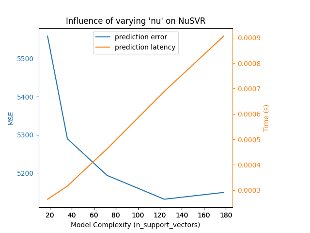
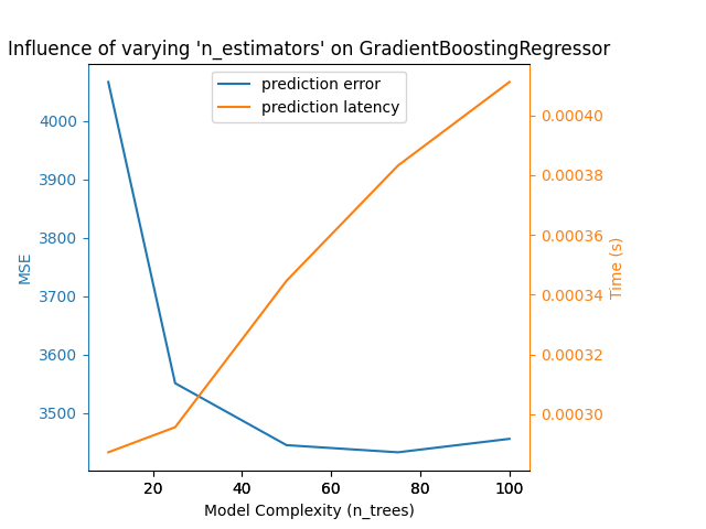
قمنا بتعريف جميع الدوال المطلوبة لتشغيل معيارنا. الآن، سنقوم بالدوران على التكوينات المختلفة التي قمنا بتعريفها مسبقًا. بعد ذلك، يمكننا تحليل الرسوم البيانية التي تم الحصول عليها من المعيار: يؤدي تخفيف عقوبة L1 في مصنف SGD إلى تقليل خطأ التنبؤ ولكن يؤدي إلى زيادة في وقت التدريب. يمكننا إجراء تحليل مماثل فيما يتعلق بوقت التدريب الذي يزيد مع عدد المتجهات الداعمة مع Nu-SVR. ومع ذلك، لاحظنا أن هناك عددًا مثاليًا من المتجهات الداعمة التي تقلل من خطأ التنبؤ. في الواقع، يؤدي عدد قليل جدًا من المتجهات الداعمة إلى نموذج غير مناسب بينما يؤدي عدد كبير جدًا من المتجهات الداعمة إلى نموذج مفرط في التكيف. يمكن استخلاص نفس الاستنتاج تمامًا للنموذج التدرج التدريجي. الفرق الوحيد مع Nu-SVR هو أن وجود عدد كبير جدًا من الأشجار في المجموعة ليس ضارًا بنفس القدر.

def plot_influence(conf, mse_values, prediction_times, complexities):
    """
    رسم تأثير تعقيد النموذج على كل من الدقة والاستجابة.
    """

    fig = plt.figure()
    fig.subplots_adjust(right=0.75)

    # المحاور الأولى (خطأ التنبؤ)
    ax1 = fig.add_subplot(111)
    line1 = ax1.plot(complexities, mse_values, c="tab:blue", ls="-")[0]
    ax1.set_xlabel("Model Complexity (%s)" % conf["complexity_label"])
    y1_label = conf["prediction_performance_label"]
    ax1.set_ylabel(y1_label)

    ax1.spines["left"].set_color(line1.get_color())
    ax1.yaxis.label.set_color(line1.get_color())
    ax1.tick_params(axis="y", colors=line1.get_color())

    # المحاور الثانية (الاستجابة)
    ax2 = fig.add_subplot(111, sharex=ax1, frameon=False)
    line2 = ax2.plot(complexities, prediction_times, c="tab:orange", ls="-")[0]
    ax2.yaxis.tick_right()
    ax2.yaxis.set_label_position("right")
    y2_label = "Time (s)"
    ax2.set_ylabel(y2_label)
    ax1.spines["right"].set_color(line2.get_color())
    ax2.yaxis.label.set_color(line2.get_color())
    ax2.tick_params(axis="y", colors=line2.get_color())

    plt.legend(
        (line1, line2), ("prediction error", "prediction latency"), loc="upper center"
    )

    plt.title(
        "Influence of varying '%s' on %s"
        % (conf["changing_param"], conf["estimator"].__name__)
    )


for conf in configurations:
    prediction_performances, prediction_times, complexities = benchmark_influence(
        conf)
    plot_influence(conf, prediction_performances,
                   prediction_times, complexities)
plt.show()

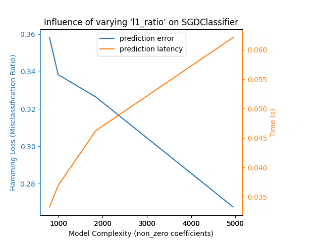
Benchmarking SGDClassifier(alpha=0.001, l1_ratio=0.25, loss='modified_huber',
              n_iter_no_change=2, penalty='elasticnet', tol=0.1)
Complexity: 4948 | Hamming Loss (Misclassification Ratio): 0.2675 | Pred. Time: 0.062088s

Benchmarking SGDClassifier(alpha=0.001, l1_ratio=0.5, loss='modified_huber',
              n_iter_no_change=2, penalty='elasticnet', tol=0.1)
Complexity: 1847 | Hamming Loss (Misclassification Ratio): 0.3264 | Pred. Time: 0.046257s

Benchmarking SGDClassifier(alpha=0.001, l1_ratio=0.75, loss='modified_huber',
              n_iter_no_change=2, penalty='elasticnet', tol=0.1)
Complexity: 997 | Hamming Loss (Misclassification Ratio): 0.3383 | Pred. Time: 0.036946s

Benchmarking SGDClassifier(alpha=0.001, l1_ratio=0.9, loss='modified_huber',
              n_iter_no_change=2, penalty='elasticnet', tol=0.1)
Complexity: 802 | Hamming Loss (Misclassification Ratio): 0.3582 | Pred. Time: 0.033295s

Benchmarking NuSVR(C=1000.0, gamma=3.0517578125e-05, nu=0.05)
Complexity: 18 | MSE: 5558.7313 | Pred. Time: 0.000265s

Benchmarking NuSVR(C=1000.0, gamma=3.0517578125e-05, nu=0.1)
Complexity: 36 | MSE: 5289.8022 | Pred. Time: 0.000316s

Benchmarking NuSVR(C=1000.0, gamma=3.0517578125e-05, nu=0.2)
Complexity: 72 | MSE: 5193.8353 | Pred. Time: 0.000463s

Benchmarking NuSVR(C=1000.0, gamma=3.0517578125e-05, nu=0.35)
Complexity: 124 | MSE: 5131.3279 | Pred. Time: 0.000689s

Benchmarking NuSVR(C=1000.0, gamma=3.0517578125e-05)
Complexity: 178 | MSE: 5149.0779 | Pred. Time: 0.000906s

Benchmarking GradientBoostingRegressor(learning_rate=0.05, max_depth=2, n_estimators=10)
Complexity: 10 | MSE: 4066.4812 | Pred. Time: 0.000287s

Benchmarking GradientBoostingRegressor(learning_rate=0.05, max_depth=2, n_estimators=25)
Complexity: 25 | MSE: 3551.1723 | Pred. Time: 0.000296s

Benchmarking GradientBoostingRegressor(learning_rate=0.05, max_depth=2, n_estimators=50)
Complexity: 50 | MSE: 3445.2171 | Pred. Time: 0.000345s

Benchmarking GradientBoostingRegressor(learning_rate=0.05, max_depth=2, n_estimators=75)
Complexity: 75 | MSE: 3433.0358 | Pred. Time: 0.000383s

Benchmarking GradientBoostingRegressor(learning_rate=0.05, max_depth=2)
Complexity: 100 | MSE: 3456.0602 | Pred. Time: 0.000411s