ملاحظة

Go to the end to download the full example code. or to run this example in your browser via JupyterLite or Binder

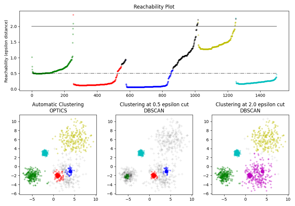
عرض توضيحي لخوارزمية التجميع OPTICS#

يحدد العينات الأساسية ذات الكثافة العالية ويوسع التجمعات منها. يستخدم هذا المثال بيانات تم إنشاؤها بحيث يكون للتجمعات كثافات مختلفة.

يتم استخدام OPTICS أولاً مع طريقة اكتشاف التجمعات Xi الخاصة به، ثم تعيين عتبات محددة على إمكانية الوصول، والتي تتوافق مع DBSCAN. يمكننا أن نرى أن التجمعات المختلفة لطريقة Xi في OPTICS يمكن استردادها مع خيارات مختلفة العتبات في DBSCAN.

Reachability Plot, Automatic Clustering OPTICS, Clustering at 0.5 epsilon cut DBSCAN, Clustering at 2.0 epsilon cut DBSCAN

# المؤلفون: مطوري scikit-learn
# تعريف الترخيص: BSD-3-Clause

import matplotlib.gridspec as gridspec
import matplotlib.pyplot as plt
import numpy as np

from sklearn.cluster import OPTICS, cluster_optics_dbscan

# توليد بيانات العينة

np.random.seed(0)
n_points_per_cluster = 250

C1 = [-5, -2] + 0.8 * np.random.randn(n_points_per_cluster, 2)
C2 = [4, -1] + 0.1 * np.random.randn(n_points_per_cluster, 2)
C3 = [1, -2] + 0.2 * np.random.randn(n_points_per_cluster, 2)
C4 = [-2, 3] + 0.3 * np.random.randn(n_points_per_cluster, 2)
C5 = [3, -2] + 1.6 * np.random.randn(n_points_per_cluster, 2)
C6 = [5, 6] + 2 * np.random.randn(n_points_per_cluster, 2)
X = np.vstack((C1, C2, C3, C4, C5, C6))

clust = OPTICS(min_samples=50, xi=0.05, min_cluster_size=0.05)

# Run the fit
clust.fit(X)

labels_050 = cluster_optics_dbscan(
    reachability=clust.reachability_,
    core_distances=clust.core_distances_,
    ordering=clust.ordering_,
    eps=0.5,
)
labels_200 = cluster_optics_dbscan(
    reachability=clust.reachability_,
    core_distances=clust.core_distances_,
    ordering=clust.ordering_,
    eps=2,
)

space = np.arange(len(X))
reachability = clust.reachability_[clust.ordering_]
labels = clust.labels_[clust.ordering_]

plt.figure(figsize=(10, 7))
G = gridspec.GridSpec(2, 3)
ax1 = plt.subplot(G[0, :])
ax2 = plt.subplot(G[1, 0])
ax3 = plt.subplot(G[1, 1])
ax4 = plt.subplot(G[1, 2])

# Reachability plot
colors = ["g.", "r.", "b.", "y.", "c."]
for klass, color in enumerate(colors):
    Xk = space[labels == klass]
    Rk = reachability[labels == klass]
    ax1.plot(Xk, Rk, color, alpha=0.3)
ax1.plot(space[labels == -1], reachability[labels == -1], "k.", alpha=0.3)
ax1.plot(space, np.full_like(space, 2.0, dtype=float), "k-", alpha=0.5)
ax1.plot(space, np.full_like(space, 0.5, dtype=float), "k-.", alpha=0.5)
ax1.set_ylabel("Reachability (epsilon distance)")
ax1.set_title("Reachability Plot")

# OPTICS
colors = ["g.", "r.", "b.", "y.", "c."]
for klass, color in enumerate(colors):
    Xk = X[clust.labels_ == klass]
    ax2.plot(Xk[:, 0], Xk[:, 1], color, alpha=0.3)
ax2.plot(X[clust.labels_ == -1, 0], X[clust.labels_ == -1, 1], "k+", alpha=0.1)
ax2.set_title("Automatic Clustering\nOPTICS")

# DBSCAN at 0.5
colors = ["g.", "r.", "b.", "c."]
for klass, color in enumerate(colors):
    Xk = X[labels_050 == klass]
    ax3.plot(Xk[:, 0], Xk[:, 1], color, alpha=0.3)
ax3.plot(X[labels_050 == -1, 0], X[labels_050 == -1, 1], "k+", alpha=0.1)
ax3.set_title("Clustering at 0.5 epsilon cut\nDBSCAN")

# DBSCAN at 2.
colors = ["g.", "m.", "y.", "c."]
for klass, color in enumerate(colors):
    Xk = X[labels_200 == klass]
    ax4.plot(Xk[:, 0], Xk[:, 1], color, alpha=0.3)
ax4.plot(X[labels_200 == -1, 0], X[labels_200 == -1, 1], "k+", alpha=0.1)
ax4.set_title("Clustering at 2.0 epsilon cut\nDBSCAN")

plt.tight_layout()
plt.show()