ملاحظة
Go to the end to download the full example code. or to run this example in your browser via JupyterLite or Binder
اختيار الميزة أحادية المتغير#
هذا الدفتر هو مثال على استخدام اختيار الميزات أحادي المتغير لتحسين دقة التصنيف على مجموعة بيانات صاخبة.
في هذا المثال، تتم إضافة بعض الميزات الصاخبة (غير المعلوماتية) إلى مجموعة بيانات iris. يتم استخدام آلة متجه الدعم (SVM) لتصنيف مجموعة البيانات قبل وبعد تطبيق اختيار الميزات أحادي المتغير. لكل ميزة، نرسم قيم p لاختيار الميزات أحادي المتغير والأوزان المقابلة لـ SVMs. مع هذا، سنقارن دقة النموذج ونفحص تأثير اختيار الميزات أحادي المتغير على أوزان النموذج.
# Authors: The scikit-learn developers
# SPDX-License-Identifier: BSD-3-Clause
توليد بيانات العينة#
import numpy as np

from sklearn.datasets import load_iris
from sklearn.model_selection import train_test_split

# The iris dataset
X, y = load_iris(return_X_y=True)

# Some noisy data not correlated
E = np.random.RandomState(42).uniform(0, 0.1, size=(X.shape[0], 20))

# Add the noisy data to the informative features
X = np.hstack((X, E))

# Split dataset to select feature and evaluate the classifier
X_train, X_test, y_train, y_test = train_test_split(X, y, stratify=y, random_state=0)
اختيار الميزات أحادي المتغير#
اختيار الميزات أحادي المتغير مع اختبار F لتسجيل الميزات. نستخدم دالة الاختيار الافتراضية لتحديد أهم أربع ميزات.
from sklearn.feature_selection import SelectKBest, f_classif

selector = SelectKBest(f_classif, k=4)
selector.fit(X_train, y_train)
scores = -np.log10(selector.pvalues_)
scores /= scores.max()
import matplotlib.pyplot as plt

X_indices = np.arange(X.shape[-1])
plt.figure(1)
plt.clf()
plt.bar(X_indices - 0.05, scores, width=0.2)
plt.title("درجة الميزة أحادية المتغير")
plt.xlabel("رقم الميزة")
plt.ylabel(r"Univariate score ($-Log(p_{value})$)")
plt.show()
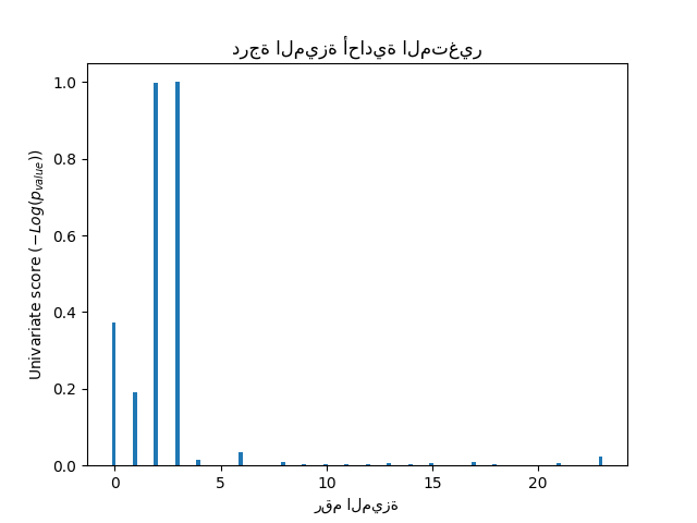
في المجموعة الكلية من الميزات، فقط 4 من الميزات الأصلية مهمة. يمكننا أن نرى أن لديهم أعلى درجة مع اختيار الميزات أحادي المتغير.
المقارنة مع SVMs#
بدون اختيار الميزات أحادي المتغير
from sklearn.pipeline import make_pipeline
from sklearn.preprocessing import MinMaxScaler
from sklearn.svm import LinearSVC

clf = make_pipeline(MinMaxScaler(), LinearSVC())
clf.fit(X_train, y_train)
print(
    "دقة التصنيف بدون اختيار الميزات: {:.3f}".format(
        clf.score(X_test, y_test)
    )
)

svm_weights = np.abs(clf[-1].coef_).sum(axis=0)
svm_weights /= svm_weights.sum()
دقة التصنيف بدون اختيار الميزات: 0.789
بعد اختيار الميزات أحادي المتغير
clf_selected = make_pipeline(SelectKBest(f_classif, k=4), MinMaxScaler(), LinearSVC())
clf_selected.fit(X_train, y_train)
print(
    "دقة التصنيف بعد اختيار الميزات أحادي المتغير: {:.3f}".format(
        clf_selected.score(X_test, y_test)
    )
)

svm_weights_selected = np.abs(clf_selected[-1].coef_).sum(axis=0)
svm_weights_selected /= svm_weights_selected.sum()
دقة التصنيف بعد اختيار الميزات أحادي المتغير: 0.868
plt.bar(
    X_indices - 0.45, scores, width=0.2, label=r"Univariate score ($-Log(p_{value})$)"
)

plt.bar(X_indices - 0.25, svm_weights, width=0.2, label="SVM weight")

plt.bar(
    X_indices[selector.get_support()] - 0.05,
    svm_weights_selected,
    width=0.2,
    label="SVM weights after selection",
)

plt.title("مقارنة اختيار الميزات")
plt.xlabel("رقم الميزة")
plt.yticks(())
plt.axis("tight")
plt.legend(loc="upper right")
plt.show()
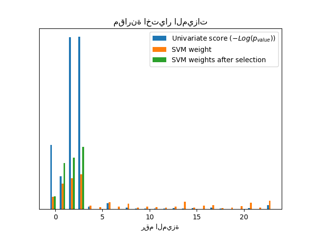
بدون اختيار الميزات أحادي المتغير، تعين SVM وزنًا كبيرًا لأول 4 ميزات أصلية مهمة، ولكنها تختار أيضًا العديد من الميزات غير المعلوماتية. تطبيق اختيار الميزات أحادي المتغير قبل SVM يزيد من وزن SVM المنسوب إلى الميزات المهمة، وبالتالي سيحسن التصنيف.
Total running time of the script: (0 minutes 0.327 seconds)
Related examples

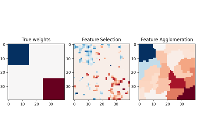
sphx_glr_auto_examples_cluster_plot_feature_agglomeration_vs_univariate_selection.py