ملاحظة

Go to the end to download the full example code. or to run this example in your browser via JupyterLite or Binder

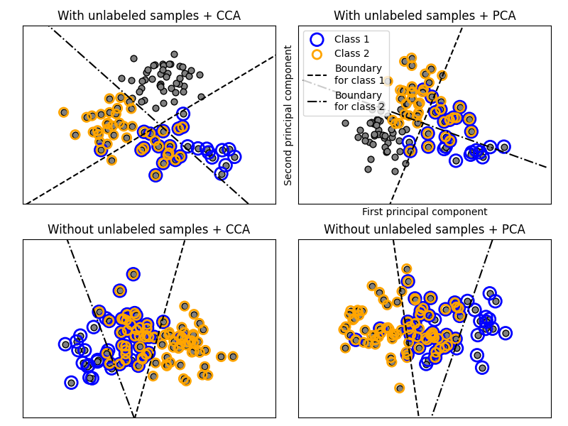
التصنيف متعدد التصنيفات#

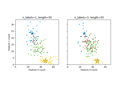
هذا المثال يحاكي مشكلة تصنيف المستندات متعددة التصنيفات. يتم توليد مجموعة البيانات بشكل عشوائي بناءً على العملية التالية:

اختيار عدد التصنيفات: n ~ Poisson(n_labels)
n مرات، اختيار تصنيف c: c ~ Multinomial(theta)
اختيار طول المستند: k ~ Poisson(length)
k مرات، اختيار كلمة: w ~ Multinomial(theta_c)

في العملية أعلاه، يتم استخدام عينة الرفض لضمان أن n أكبر من 2، وأن طول المستند لا يكون أبدًا صفرًا. وبالمثل، نرفض التصنيفات التي تم اختيارها بالفعل. يتم تمثيل المستندات التي تم تعيينها لكلا التصنيفين محاطة بدائرتين ملونتين.

يتم تنفيذ التصنيف من خلال إسقاطه على أول مكونين رئيسيين تم العثور عليهما بواسطة PCA وCCA لأغراض العرض المرئي، يليه استخدام التصنيف الفائق OneVsRestClassifier باستخدام SVCs مع نوى خطية لتعلم نموذج تمييزي لكل تصنيف. ملاحظة: يتم استخدام PCA لإجراء تقليل أبعاد غير مشرف، بينما يتم استخدام CCA لإجراء تقليل أبعاد مشرف.

ملاحظة: في الرسم البياني، لا تعني "العينات غير المصنفة" أننا لا نعرف التصنيفات (كما في التعلم شبه المشرف)، ولكن أن العينات ببساطة لا تحتوي على تصنيف.

With unlabeled samples + CCA, With unlabeled samples + PCA, Without unlabeled samples + CCA, Without unlabeled samples + PCA

# المؤلفون: مطوري scikit-learn
# معرف الترخيص: BSD-3-Clause

import matplotlib.pyplot as plt
import numpy as np

from sklearn.cross_decomposition import CCA
from sklearn.datasets import make_multilabel_classification
from sklearn.decomposition import PCA
from sklearn.multiclass import OneVsRestClassifier
from sklearn.svm import SVC


def plot_hyperplane(clf, min_x, max_x, linestyle, label):
    # الحصول على المستوي الفاصل
    w = clf.coef_[0]
    a = -w[0] / w[1]
    xx = np.linspace(min_x - 5, max_x + 5)  # التأكد من أن الخط طويل بما يكفي
    yy = a * xx - (clf.intercept_[0]) / w[1]
    plt.plot(xx, yy, linestyle, label=label)


def plot_subfigure(X, Y, subplot, title, transform):
    if transform == "pca":
        X = PCA(n_components=2).fit_transform(X)
    elif transform == "cca":
        X = CCA(n_components=2).fit(X, Y).transform(X)
    else:
        raise ValueError

    min_x = np.min(X[:, 0])
    max_x = np.max(X[:, 0])

    min_y = np.min(X[:, 1])
    max_y = np.max(X[:, 1])

    classif = OneVsRestClassifier(SVC(kernel="linear"))
    classif.fit(X, Y)

    plt.subplot(2, 2, subplot)
    plt.title(title)

    zero_class = np.where(Y[:, 0])
    one_class = np.where(Y[:, 1])
    plt.scatter(X[:, 0], X[:, 1], s=40, c="gray", edgecolors=(0, 0, 0))
    plt.scatter(
        X[zero_class, 0],
        X[zero_class, 1],
        s=160,
        edgecolors="b",
        facecolors="none",
        linewidths=2,
        label="Class 1",
    )
    plt.scatter(
        X[one_class, 0],
        X[one_class, 1],
        s=80,
        edgecolors="orange",
        facecolors="none",
        linewidths=2,
        label="Class 2",
    )

    plot_hyperplane(
        classif.estimators_[0], min_x, max_x, "k--", "Boundary\nfor class 1"
    )
    plot_hyperplane(
        classif.estimators_[1], min_x, max_x, "k-.", "Boundary\nfor class 2"
    )
    plt.xticks(())
    plt.yticks(())

    plt.xlim(min_x - 0.5 * max_x, max_x + 0.5 * max_x)
    plt.ylim(min_y - 0.5 * max_y, max_y + 0.5 * max_y)
    if subplot == 2:
        plt.xlabel("First principal component")
        plt.ylabel("Second principal component")
        plt.legend(loc="upper left")


plt.figure(figsize=(8, 6))

X, Y = make_multilabel_classification(
    n_classes=2, n_labels=1, allow_unlabeled=True, random_state=1
)

plot_subfigure(X, Y, 1, "With unlabeled samples + CCA", "cca")
plot_subfigure(X, Y, 2, "With unlabeled samples + PCA", "pca")

X, Y = make_multilabel_classification(
    n_classes=2, n_labels=1, allow_unlabeled=False, random_state=1
)

plot_subfigure(X, Y, 3, "Without unlabeled samples + CCA", "cca")
plot_subfigure(X, Y, 4, "Without unlabeled samples + PCA", "pca")

plt.subplots_adjust(0.04, 0.02, 0.97, 0.94, 0.09, 0.2)
plt.show()