ملاحظة
Go to the end to download the full example code. or to run this example in your browser via JupyterLite or Binder
اختيار النموذج باستخدام التحليل الرئيسي للمكونات الاحتمالي وتحليل العوامل (FA)#
التحليل الرئيسي للمكونات الاحتمالي وتحليل العوامل هما نموذجان احتماليان. والنتيجة هي أنه يمكن استخدام احتمالية البيانات الجديدة لاختيار النموذج وتقدير التباين. هنا نقارن بين التحليل الرئيسي للمكونات وتحليل العوامل باستخدام التحقق المتقاطع على البيانات منخفضة الرتبة التي تتعرض للتشويش بضوضاء متماثلة (تكون تباين الضوضاء نفس الشيء لكل ميزة) أو الضوضاء غير المتماثلة (تكون تباين الضوضاء مختلفًا لكل ميزة). في الخطوة الثانية، نقارن بين نموذج الاحتمالية مع الاحتمالات التي تم الحصول عليها من مقدرات التباين الانكماشي.
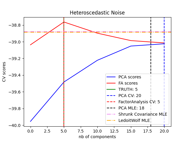
يمكن ملاحظة أنه مع الضوضاء المتماثلة، ينجح كل من تحليل العوامل والتحليل الرئيسي للمكونات في استعادة حجم الفضاء منخفض الرتبة. الاحتمالية مع التحليل الرئيسي للمكونات أعلى من تحليل العوامل في هذه الحالة. ومع ذلك، يفشل التحليل الرئيسي للمكونات ويبالغ في تقدير الرتبة عند وجود ضوضاء غير متماثلة. في ظل الظروف المناسبة (اختيار عدد المكونات)، البيانات المحجوبة من المرجح أن تكون أكثر انخفاضًا في نماذج الرتبة من نماذج الانكماش.
يتم أيضًا مقارنة التقدير التلقائي من الاختيار التلقائي للأبعاد للتحليل الرئيسي للمكونات. NIPS 2000: 598-604 بواسطة توماس ب. مينكا.
# المؤلفون: مطوري scikit-learn
# معرف الترخيص: BSD-3-Clause
إنشاء البيانات#
from sklearn.model_selection import GridSearchCV, cross_val_score
from sklearn.decomposition import PCA, FactorAnalysis
from sklearn.covariance import LedoitWolf, ShrunkCovariance
import matplotlib.pyplot as plt
import numpy as np
from scipy import linalg

n_samples, n_features, rank = 500, 25, 5
sigma = 1.0
rng = np.random.RandomState(42)
U, _, _ = linalg.svd(rng.randn(n_features, n_features))
X = np.dot(rng.randn(n_samples, rank), U[:, :rank].T)

# إضافة ضوضاء متماثلة
X_homo = X + sigma * rng.randn(n_samples, n_features)

# إضافة ضوضاء غير متماثلة
sigmas = sigma * rng.rand(n_features) + sigma / 2.0
X_hetero = X + rng.randn(n_samples, n_features) * sigmas
ملاءمة النماذج#
n_components = np.arange(0, n_features, 5)  # الخيارات لـ n_components


def compute_scores(X):
    pca = PCA(svd_solver="full")
    fa = FactorAnalysis()

    pca_scores, fa_scores = [], []
    for n in n_components:
        pca.n_components = n
        fa.n_components = n
        pca_scores.append(np.mean(cross_val_score(pca, X)))
        fa_scores.append(np.mean(cross_val_score(fa, X)))

    return pca_scores, fa_scores


def shrunk_cov_score(X):
    shrinkages = np.logspace(-2, 0, 30)
    cv = GridSearchCV(ShrunkCovariance(), {"shrinkage": shrinkages})
    return np.mean(cross_val_score(cv.fit(X).best_estimator_, X))


def lw_score(X):
    return np.mean(cross_val_score(LedoitWolf(), X))


for X, title in [(X_homo, "Homoscedastic Noise"), (X_hetero, "Heteroscedastic Noise")]:
    pca_scores, fa_scores = compute_scores(X)
    n_components_pca = n_components[np.argmax(pca_scores)]
    n_components_fa = n_components[np.argmax(fa_scores)]

    pca = PCA(svd_solver="full", n_components="mle")
    pca.fit(X)
    n_components_pca_mle = pca.n_components_

    print("best n_components by PCA CV = %d" % n_components_pca)
    print("best n_components by FactorAnalysis CV = %d" % n_components_fa)
    print("best n_components by PCA MLE = %d" % n_components_pca_mle)

    plt.figure()
    plt.plot(n_components, pca_scores, "b", label="PCA scores")
    plt.plot(n_components, fa_scores, "r", label="FA scores")
    plt.axvline(rank, color="g", label="TRUTH: %d" % rank, linestyle="-")
    plt.axvline(
        n_components_pca,
        color="b",
        label="PCA CV: %d" % n_components_pca,
        linestyle="--",
    )
    plt.axvline(
        n_components_fa,
        color="r",
        label="FactorAnalysis CV: %d" % n_components_fa,
        linestyle="--",
    )
    plt.axvline(
        n_components_pca_mle,
        color="k",
        label="PCA MLE: %d" % n_components_pca_mle,
        linestyle="--",
    )
# compare with other covariance estimators
    plt.axhline(
        shrunk_cov_score(X),
        color="violet",
        label="Shrunk Covariance MLE",
        linestyle="-.",
    )
    plt.axhline(
        lw_score(X),
        color="orange",
        label="LedoitWolf MLE" % n_components_pca_mle,
        linestyle="-.",
    )

    plt.xlabel("nb of components")
    plt.ylabel("CV scores")
    plt.legend(loc="lower right")
    plt.title(title)

plt.show()
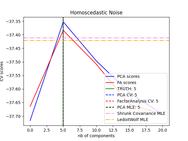
best n_components by PCA CV = 5
best n_components by FactorAnalysis CV = 5
best n_components by PCA MLE = 5
best n_components by PCA CV = 20
best n_components by FactorAnalysis CV = 5
best n_components by PCA MLE = 18
Total running time of the script: (0 minutes 3.868 seconds)
Related examples
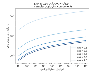
حدود جونسون-ليندستراوس للانغماس مع الإسقاطات العشوائية
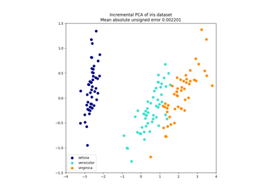
sphx_glr_auto_examples_decomposition_plot_incremental_pca.py