تصنيف وثائق النصوص باستخدام الميزات المتناثرة

هذا مثال يوضح كيفية استخدام scikit-learn لتصنيف الوثائق حسب الموضوعات باستخدام نهج "Bag of Words" <https://en.wikipedia.org/wiki/Bag-of-words_model>_. يستخدم هذا المثال مصفوفة متقطعة ذات وزن Tf-idf لتشفير الميزات ويظهر العديد من التصنيفات التي يمكنها التعامل بكفاءة مع المصفوفات المتقطعة.

لتحليل الوثائق عبر نهج التعلم غير الخاضع للإشراف، راجع مثال النص تجميع مستندات النص باستخدام k-means.

# المؤلفون: مطوري scikit-learn
# معرف SPDX-License: BSD-3-Clause

تحميل وتجهيز مجموعة بيانات 20 newsgroups النصية

نحن نحدد وظيفة لتحميل البيانات من The 20 newsgroups text dataset، والتي تتكون من حوالي 18000 مشاركة في مجموعات الأخبار حول 20 موضوع مقسمة إلى مجموعتين: واحدة للتدريب (أو التطوير) والأخرى للاختبار (أو لتقييم الأداء). لاحظ أنه، بشكل افتراضي، تحتوي عينات النص على بعض بيانات التعريف مثل 'headers'، 'footers' (التوقيعات) و 'quotes' إلى المشاركات الأخرى. لذلك، تقبل وظيفة fetch_20newsgroups معلمة تسمى remove لمحاولة إزالة مثل هذه المعلومات التي يمكن أن تجعل مشكلة التصنيف "سهلة للغاية". يتم تحقيق ذلك باستخدام خوارزميات بسيطة ليست مثالية ولا معيارية، وبالتالي يتم تعطيلها بشكل افتراضي.

from time import time

from sklearn.datasets import fetch_20newsgroups
from sklearn.feature_extraction.text import TfidfVectorizer

categories = [
    "alt.atheism",
    "talk.religion.misc",
    "comp.graphics",
    "sci.space",
]


def size_mb(docs):
    return sum(len(s.encode("utf-8")) for s in docs) / 1e6


def load_dataset(verbose=False, remove=()):
    """تحميل وتجهيز مجموعة بيانات 20 newsgroups."""

    data_train = fetch_20newsgroups(
        subset="train",
        categories=categories,
        shuffle=True,
        random_state=42,
        remove=remove,
    )

    data_test = fetch_20newsgroups(
        subset="test",
        categories=categories,
        shuffle=True,
        random_state=42,
        remove=remove,
    )

    # يمكن أن يختلف ترتيب التصنيفات في `target_names` عن `categories`
    target_names = data_train.target_names

    # تقسيم التصنيفات إلى مجموعة تدريب ومجموعة اختبار
    y_train, y_test = data_train.target, data_test.target

    # استخراج الميزات من بيانات التدريب باستخدام متجه متقطع
    t0 = time()
    vectorizer = TfidfVectorizer(
        sublinear_tf=True, max_df=0.5, min_df=5, stop_words="english"
    )
    X_train = vectorizer.fit_transform(data_train.data)
    duration_train = time() - t0

    # استخراج الميزات من بيانات الاختبار باستخدام نفس المتجه
    t0 = time()
    X_test = vectorizer.transform(data_test.data)
    duration_test = time() - t0

    feature_names = vectorizer.get_feature_names_out()

    if verbose:
        # حساب حجم البيانات المحملة
        data_train_size_mb = size_mb(data_train.data)
        data_test_size_mb = size_mb(data_test.data)

        print(
            f"{len(data_train.data)} documents - "
            f"{data_train_size_mb:.2f}MB (training set)"
        )
        print(f"{len(data_test.data)} documents - {data_test_size_mb:.2f}MB (test set)")
        print(f"{len(target_names)} categories")
        print(
            f"vectorize training done in {duration_train:.3f}s "
            f"at {data_train_size_mb / duration_train:.3f}MB/s"
        )
        print(f"n_samples: {X_train.shape[0]}, n_features: {X_train.shape[1]}")
        print(
            f"vectorize testing done in {duration_test:.3f}s "
            f"at {data_test_size_mb / duration_test:.3f}MB/s"
        )
        print(f"n_samples: {X_test.shape[0]}, n_features: {X_test.shape[1]}")

    return X_train, X_test, y_train, y_test, feature_names, target_names

تحليل مصنف وثائق Bag-of-words

سنقوم الآن بتدريب مصنف مرتين، مرة على عينات النص بما في ذلك بيانات التعريف ومرة أخرى بعد إزالة بيانات التعريف. بالنسبة لكلتا الحالتين، سنقوم بتحليل أخطاء التصنيف على مجموعة اختبار باستخدام مصفوفة الارتباك وفحص المعاملات التي تحدد وظيفة التصنيف للنماذج المدربة.

النموذج بدون إزالة بيانات التعريف

نبدأ باستخدام الوظيفة المخصصة load_dataset لتحميل البيانات بدون إزالة بيانات التعريف.

X_train, X_test, y_train, y_test, feature_names, target_names = load_dataset(
    verbose=True
)

2034 documents - 3.98MB (training set)
1353 documents - 2.87MB (test set)
4 categories
vectorize training done in 0.452s at 8.812MB/s
n_samples: 2034, n_features: 7831
vectorize testing done in 0.320s at 8.972MB/s
n_samples: 1353, n_features: 7831

نموذجنا الأول هو مثيل لفئة RidgeClassifier. هذا هو نموذج التصنيف الخطي الذي يستخدم متوسط خطأ المربعات على الأهداف المشفرة {-1, 1}، واحد لكل فئة ممكنة. على عكس LogisticRegression، RidgeClassifier لا يوفر تنبؤات احتمالية (لا توجد طريقة predict_proba)، ولكنها غالبًا ما تكون أسرع في التدريب.

from sklearn.linear_model import RidgeClassifier

clf = RidgeClassifier(tol=1e-2, solver="sparse_cg")
clf.fit(X_train, y_train)
pred = clf.predict(X_test)

نرسم مصفوفة الارتباك لهذا المصنف لمعرفة ما إذا كان هناك نمط في أخطاء التصنيف.

import matplotlib.pyplot as plt

from sklearn.metrics import ConfusionMatrixDisplay

fig, ax = plt.subplots(figsize=(10, 5))
ConfusionMatrixDisplay.from_predictions(y_test, pred, ax=ax)
ax.xaxis.set_ticklabels(target_names)
ax.yaxis.set_ticklabels(target_names)
_ = ax.set_title(
    f"Confusion Matrix for {clf.__class__.__name__}\non the original documents"
)

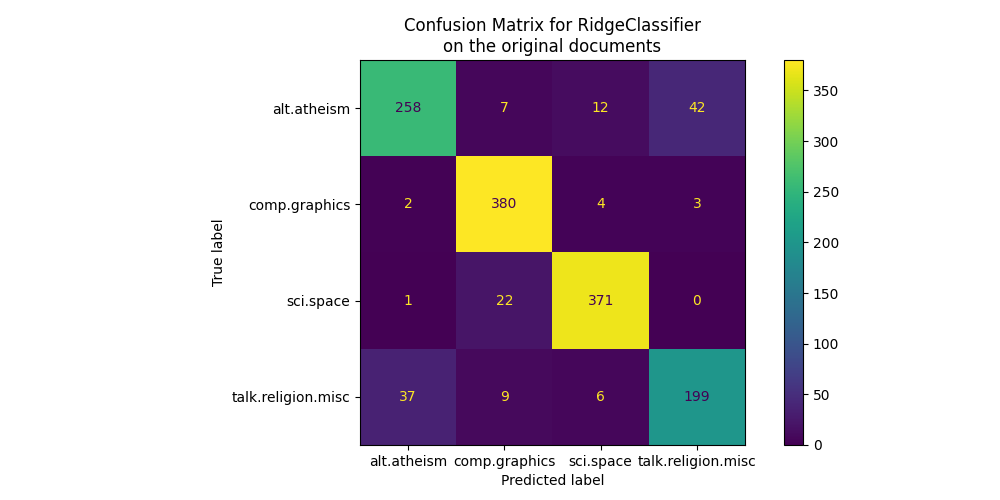
تسلط مصفوفة الارتباك الضوء على أن وثائق فئة alt.atheism غالبًا ما يتم الخلط بينها مع وثائق فئة talk.religion.misc والعكس صحيح، وهو ما كان متوقعًا لأن الموضوعات ذات صلة دلاليًا.

نلاحظ أيضًا أن بعض وثائق فئة sci.space يمكن أن يتم تصنيفها بشكل خاطئ على أنها comp.graphics في حين أن العكس نادر جدًا. سيتطلب الفحص اليدوي لتلك الوثائق المصنفة بشكل سيء بعض الأفكار حول هذا عدم التناسق. قد يكون من الممكن أن تكون المفردات الخاصة بموضوع الفضاء أكثر تحديدًا من المفردات الخاصة بالرسومات الحاسوبية.

يمكننا اكتساب فهم أعمق لكيفية اتخاذ هذا المصنف لقراراته من خلال النظر إلى الكلمات ذات أعلى متوسط تأثيرات الميزات:

import numpy as np
import pandas as pd


def plot_feature_effects():
    # المعاملات المكتسبة المرجحة بتردد الظهور
    average_feature_effects = clf.coef_ * np.asarray(X_train.mean(axis=0)).ravel()

    for i, label in enumerate(target_names):
        top5 = np.argsort(average_feature_effects[i])[-5:][::-1]
        if i == 0:
            top = pd.DataFrame(feature_names[top5], columns=[label])
            top_indices = top5
        else:
            top[label] = feature_names[top5]
            top_indices = np.concatenate((top_indices, top5), axis=None)
    top_indices = np.unique(top_indices)
    predictive_words = feature_names[top_indices]

    # رسم تأثيرات الميزات
    bar_size = 0.25
    padding = 0.75
    y_locs = np.arange(len(top_indices)) * (4 * bar_size + padding)

    fig, ax = plt.subplots(figsize=(10, 8))
    for i, label in enumerate(target_names):
        ax.barh(
            y_locs + (i - 2) * bar_size,
            average_feature_effects[i, top_indices],
            height=bar_size,
            label=label,
        )
    ax.set(
        yticks=y_locs,
        yticklabels=predictive_words,
        ylim=[
            0 - 4 * bar_size,
            len(top_indices) * (4 * bar_size + padding) - 4 * bar_size,
        ],
    )
    ax.legend(loc="lower right")

    print("top 5 keywords per class:")
    print(top)

    return ax


_ = plot_feature_effects().set_title("Average feature effect on the original data")

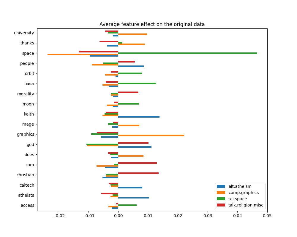
top 5 keywords per class:
  alt.atheism comp.graphics sci.space talk.religion.misc
0       keith      graphics     space          christian
1         god    university      nasa                com
2    atheists        thanks     orbit                god
3      people          does      moon           morality
4     caltech         image    access             people

يمكننا ملاحظة أن الكلمات الأكثر تنبؤًا غالبًا ما تكون مرتبطة إيجابيًا بقوة بفئة واحدة ومرتبطة سلبًا بجميع الفئات الأخرى. معظم هذه الارتباطات الإيجابية سهلة التفسير. ومع ذلك، هناك كلمات مثل "god" و "people" مرتبطة إيجابيًا بكل من "talk.misc.religion" و "alt.atheism" حيث من المتوقع أن تشترك هاتان الفئتان في بعض المفردات المشتركة. لاحظ مع ذلك أن هناك أيضًا كلمات مثل "christian" و "morality" التي ترتبط إيجابيًا فقط بفئة "talk.misc.religion". علاوة على ذلك، في هذه النسخة من مجموعة البيانات، فإن كلمة "caltech" هي إحدى الميزات التنبؤية العليا للإلحاد بسبب التلوث في مجموعة البيانات القادم من نوع من بيانات التعريف مثل عناوين البريد الإلكتروني للمرسل من رسائل البريد الإلكتروني السابقة في المناقشة كما هو موضح أدناه:

data_train = fetch_20newsgroups(
    subset="train", categories=categories, shuffle=True, random_state=42
)

for doc in data_train.data:
    if "caltech" in doc:
        print(doc)
        break

From: livesey@solntze.wpd.sgi.com (Jon Livesey)
Subject: Re: Morality? (was Re: <Political Atheists?)
Organization: sgi
Lines: 93
Distribution: world
NNTP-Posting-Host: solntze.wpd.sgi.com

In article <1qlettINN8oi@gap.caltech.edu>, keith@cco.caltech.edu (Keith Allan Schneider) writes:
|> livesey@solntze.wpd.sgi.com (Jon Livesey) writes:
|>
|> >>>Explain to me
|> >>>how instinctive acts can be moral acts, and I am happy to listen.
|> >>For example, if it were instinctive not to murder...
|> >
|> >Then not murdering would have no moral significance, since there
|> >would be nothing voluntary about it.
|>
|> See, there you go again, saying that a moral act is only significant
|> if it is "voluntary."  Why do you think this?

If you force me to do something, am I morally responsible for it?

|>
|> And anyway, humans have the ability to disregard some of their instincts.

Well, make up your mind.    Is it to be "instinctive not to murder"
or not?

|>
|> >>So, only intelligent beings can be moral, even if the bahavior of other
|> >>beings mimics theirs?
|> >
|> >You are starting to get the point.  Mimicry is not necessarily the
|> >same as the action being imitated.  A Parrot saying "Pretty Polly"
|> >isn't necessarily commenting on the pulchritude of Polly.
|>
|> You are attaching too many things to the term "moral," I think.
|> Let's try this:  is it "good" that animals of the same species
|> don't kill each other.  Or, do you think this is right?

It's not even correct.    Animals of the same species do kill
one another.

|>
|> Or do you think that animals are machines, and that nothing they do
|> is either right nor wrong?

Sigh.   I wonder how many times we have been round this loop.

I think that instinctive bahaviour has no moral significance.
I am quite prepared to believe that higher animals, such as
primates, have the beginnings of a moral sense, since they seem
to exhibit self-awareness.

|>
|>
|> >>Animals of the same species could kill each other arbitarily, but
|> >>they don't.
|> >
|> >They do.  I and other posters have given you many examples of exactly
|> >this, but you seem to have a very short memory.
|>
|> Those weren't arbitrary killings.  They were slayings related to some
|> sort of mating ritual or whatnot.

So what?     Are you trying to say that some killing in animals
has a moral significance and some does not?   Is this your
natural morality>


|>
|> >>Are you trying to say that this isn't an act of morality because
|> >>most animals aren't intelligent enough to think like we do?
|> >
|> >I'm saying:
|> >    "There must be the possibility that the organism - it's not
|> >    just people we are talking about - can consider alternatives."
|> >
|> >It's right there in the posting you are replying to.
|>
|> Yes it was, but I still don't understand your distinctions.  What
|> do you mean by "consider?"  Can a small child be moral?  How about
|> a gorilla?  A dolphin?  A platypus?  Where is the line drawn?  Does
|> the being need to be self aware?

Are you blind?   What do you think that this sentence means?

        "There must be the possibility that the organism - it's not
        just people we are talking about - can consider alternatives."

What would that imply?

|>
|> What *do* you call the mechanism which seems to prevent animals of
|> the same species from (arbitrarily) killing each other?  Don't
|> you find the fact that they don't at all significant?

I find the fact that they do to be significant.

jon.

يمكن اعتبار مثل هذه العناوين، وتوقيعات الأقدام (واقتباسات بيانات التعريف من الرسائل السابقة) معلومات جانبية تكشف عن مجموعة الأخبار من خلال تحديد الأعضاء المسجلين، ويفضل المرء أن يتعلم مصنف النص الخاص بنا فقط من "المحتوى الرئيسي" لكل وثيقة نصية بدلاً من الاعتماد على هوية الكُتّاب المسربة.

النموذج مع إزالة بيانات التعريف

تسمح خيار remove لمجموعة بيانات 20 newsgroups في scikit-learn بمحاولة تصفية بعض بيانات التعريف هذه التي تجعل مشكلة التصنيف أسهل بشكل مصطنع. كن على دراية بأن مثل هذا تصفية محتويات النص بعيدة عن الكمال.

دعنا نحاول الاستفادة من هذا الخيار لتدريب مصنف نص لا يعتمد كثيرًا على هذا النوع من بيانات التعريف لاتخاذ قراراته:

(
    X_train,
    X_test,
    y_train,
    y_test,
    feature_names,
    target_names,
) = load_dataset(remove=("headers", "footers", "quotes"))

clf = RidgeClassifier(tol=1e-2, solver="sparse_cg")
clf.fit(X_train, y_train)
pred = clf.predict(X_test)

fig, ax = plt.subplots(figsize=(10, 5))
ConfusionMatrixDisplay.from_predictions(y_test, pred, ax=ax)
ax.xaxis.set_ticklabels(target_names)
ax.yaxis.set_ticklabels(target_names)
_ = ax.set_title(
    f"Confusion Matrix for {clf.__class__.__name__}\non filtered documents"
)

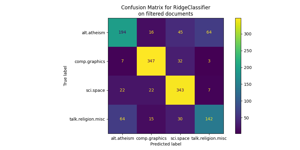
بالنظر إلى مصفوفة الارتباك، يصبح من الواضح أن درجات النموذج المدرب ببيانات التعريف كانت مفرطة في التفاؤل. مشكلة التصنيف بدون الوصول إلى بيانات التعريف أقل دقة ولكنها أكثر تمثيلاً لمشكلة تصنيف النص المقصود.

_ = plot_feature_effects().set_title("Average feature effects on filtered documents")

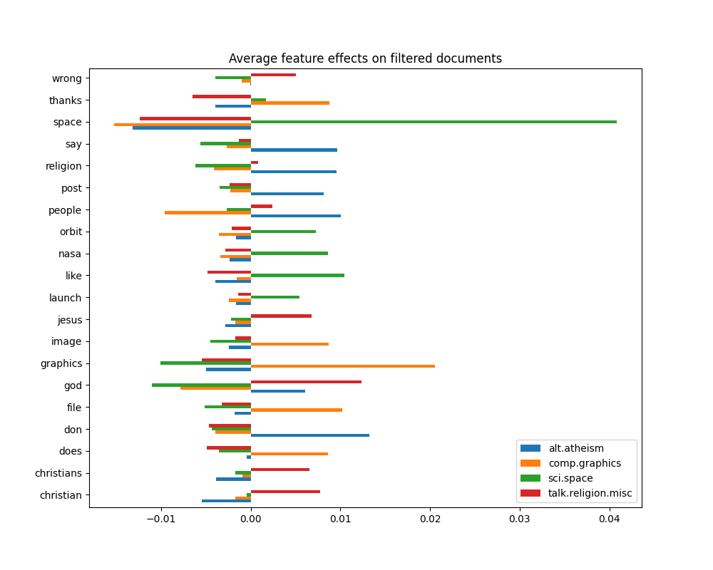
top 5 keywords per class:
  alt.atheism comp.graphics sci.space talk.religion.misc
0         don      graphics     space                god
1      people          file      like          christian
2         say        thanks      nasa              jesus
3    religion         image     orbit         christians
4        post          does    launch              wrong

في القسم التالي، سنحتفظ بمجموعة البيانات بدون بيانات التعريف لمقارنة عدة المصنفات.

اختبار أداء المصنفات

يوفر scikit-learn العديد من أنواع خوارزميات التصنيف المختلفة. في هذا القسم، سنقوم بتدريب مجموعة مختارة من هذه المصنفات على نفس مشكلة تصنيف النص وقياس كل من أداء التعميم (الدقة على مجموعة الاختبار) وأداء الحساب (السرعة)، لكل من وقت التدريب ووقت الاختبار. لهذا الغرض، نحدد المرافق التالية الأدوات:

from sklearn import metrics
from sklearn.utils.extmath import density


def benchmark(clf, custom_name=False):
    print("_" * 80)
    print("Training: ")
    print(clf)
    t0 = time()
    clf.fit(X_train, y_train)
    train_time = time() - t0
    print(f"train time: {train_time:.3}s")

    t0 = time()
    pred = clf.predict(X_test)
    test_time = time() - t0
    print(f"test time:  {test_time:.3}s")

    score = metrics.accuracy_score(y_test, pred)
    print(f"accuracy:   {score:.3}")

    if hasattr(clf, "coef_"):
        print(f"dimensionality: {clf.coef_.shape[1]}")
        print(f"density: {density(clf.coef_)}")
        print()

    print()
    if custom_name:
        clf_descr = str(custom_name)
    else:
        clf_descr = clf.__class__.__name__
    return clf_descr, score, train_time, test_time

الآن نقوم بتدريب واختبار مجموعات البيانات باستخدام 8 نماذج تصنيف مختلفة والحصول على نتائج الأداء لكل نموذج. الهدف من هذه الدراسة هو تسليط الضوء على مقايضات الحساب/الدقة لأنواع مختلفة من المصنفات لمشكلة تصنيف النص متعدد الفئات هذه.

لاحظ أن قيم أهم المعلمات تم ضبطها باستخدام إجراء البحث الشبكي غير موضح في هذا الدفتر من أجل البساطة. راجع مثال النص مثال على خط أنابيب لاستخراج ميزات النص وتقييمها # noqa: E501 للحصول على عرض توضيحي حول كيفية إجراء مثل هذا الضبط.

from sklearn.ensemble import RandomForestClassifier
from sklearn.linear_model import LogisticRegression, SGDClassifier
from sklearn.naive_bayes import ComplementNB
from sklearn.neighbors import KNeighborsClassifier, NearestCentroid
from sklearn.svm import LinearSVC

results = []
for clf, name in (
    (LogisticRegression(C=5, max_iter=1000), "الانحدار اللوجستي"),
    (RidgeClassifier(alpha=1.0, solver="sparse_cg"), "مصنف ريدج"),
    (KNeighborsClassifier(n_neighbors=100), "kNN"),
    (RandomForestClassifier(), "الغابة العشوائية"),
    # L2 penalty Linear SVC
    (LinearSVC(C=0.1, dual=False, max_iter=1000), "Linear SVC"),
    # L2 penalty Linear SGD
    (
        SGDClassifier(
            loss="log_loss", alpha=1e-4, n_iter_no_change=3, early_stopping=True
        ),
        "log-loss SGD",
    ),
    # NearestCentroid (المعروف أيضًا باسم مصنف Rocchio)
    (NearestCentroid(), "NearestCentroid"),
    # مصنف Bayes الساذج المتناثر
    (ComplementNB(alpha=0.1), "Complement naive Bayes"),
):
    print("=" * 80)
    print(name)
    results.append(benchmark(clf, name))

================================================================================
الانحدار اللوجستي
________________________________________________________________________________
Training:
LogisticRegression(C=5, max_iter=1000)
train time: 0.83s
test time:  0.00191s
accuracy:   0.772
dimensionality: 5316
density: 1.0


================================================================================
مصنف ريدج
________________________________________________________________________________
Training:
RidgeClassifier(solver='sparse_cg')
train time: 0.065s
test time:  0.0018s
accuracy:   0.76
dimensionality: 5316
density: 1.0


================================================================================
kNN
________________________________________________________________________________
Training:
KNeighborsClassifier(n_neighbors=100)
train time: 0.00208s
test time:  0.0893s
accuracy:   0.752

================================================================================
الغابة العشوائية
________________________________________________________________________________
Training:
RandomForestClassifier()
train time: 1.42s
test time:  0.0447s
accuracy:   0.689

================================================================================
Linear SVC
________________________________________________________________________________
Training:
LinearSVC(C=0.1, dual=False)
train time: 0.0246s
test time:  0.00085s
accuracy:   0.752
dimensionality: 5316
density: 1.0


================================================================================
log-loss SGD
________________________________________________________________________________
Training:
SGDClassifier(early_stopping=True, loss='log_loss', n_iter_no_change=3)
train time: 0.0432s
test time:  0.000618s
accuracy:   0.763
dimensionality: 5316
density: 1.0


================================================================================
NearestCentroid
________________________________________________________________________________
Training:
NearestCentroid()
train time: 0.0029s
test time:  0.00133s
accuracy:   0.748

================================================================================
Complement naive Bayes
________________________________________________________________________________
Training:
ComplementNB(alpha=0.1)
train time: 0.00211s
test time:  0.000508s
accuracy:   0.779

رسم دقة ووقت التدريب والاختبار لكل مصنف

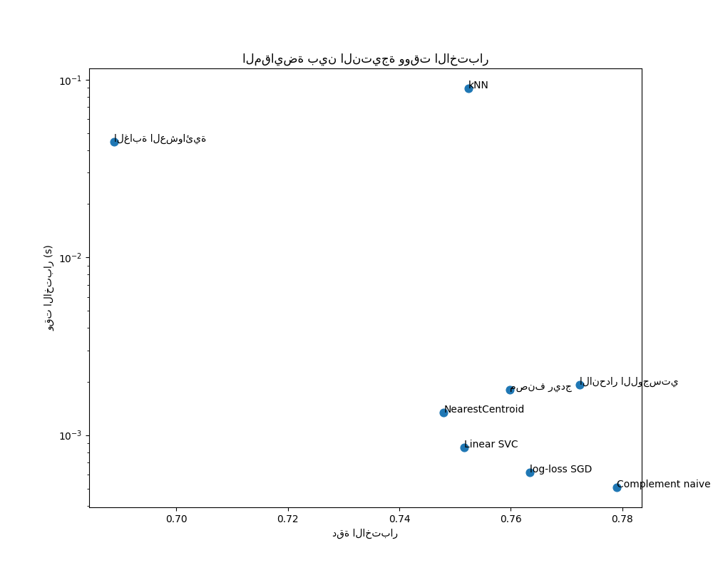
تُظهر مخططات التشتت المقايضة بين دقة الاختبار ووقت التدريب والاختبار لكل مصنف.

indices = np.arange(len(results))

results = [[x[i] for x in results] for i in range(4)]

clf_names, score, training_time, test_time = results
training_time = np.array(training_time)
test_time = np.array(test_time)

fig, ax1 = plt.subplots(figsize=(10, 8))
ax1.scatter(score, training_time, s=60)
ax1.set(
    title="المقايضة بين النتيجة ووقت التدريب",
    yscale="log",
    xlabel="دقة الاختبار",
    ylabel="وقت التدريب (s)",
)
fig, ax2 = plt.subplots(figsize=(10, 8))
ax2.scatter(score, test_time, s=60)
ax2.set(
    title="المقايضة بين النتيجة ووقت الاختبار",
    yscale="log",
    xlabel="دقة الاختبار",
    ylabel="وقت الاختبار (s)",
)


for i, txt in enumerate(clf_names):
    ax1.annotate(txt, (score[i], training_time[i]))
    ax2.annotate(txt, (score[i], test_time[i]))

• 
• 

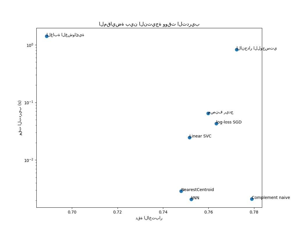
يتمتع نموذج Bayes الساذج بأفضل مقايضة بين النتيجة ووقت التدريب / الاختبار، بينما الغابة العشوائية بطيئة في التدريب، ومكلفة للتنبؤ، ولديها دقة سيئة نسبيًا. هذا متوقع: لمشاكل التنبؤ عالية الأبعاد، غالبًا ما تكون النماذج الخطية أكثر ملاءمة لأن معظم المشاكل تصبح قابلة للفصل خطيًا عندما تحتوي مساحة الميزة على 10000 بُعد أو أكثر.

يمكن تفسير الاختلاف في سرعة التدريب ودقة النماذج الخطية من خلال اختيار دالة الخسارة التي تقوم بتحسينها ونوع التنظيم الذي تستخدمه. انتبه إلى أن بعض النماذج الخطية التي لها نفس الخسارة ولكن لها مُحلل أو تكوين تنظيم مختلف قد ينتج عنها أوقات ملاءمة ودقة اختبار مختلفة. يمكننا أن نلاحظ في الرسم البياني الثاني أنه بمجرد التدريب، يكون لجميع النماذج الخطية نفس سرعة التنبؤ تقريبًا، وهو أمر متوقع لأنها جميعًا تنفذ نفس دالة التنبؤ.

يتمتع KNeighborsClassifier بدقة منخفضة نسبيًا ولديه أعلى وقت اختبار. من المتوقع أيضًا وقت التنبؤ الطويل: لكل تنبؤ، يجب على النموذج حساب المسافات الزوجية بين عينة الاختبار وكل مستند في مجموعة التدريب، وهو أمر مكلف حسابيًا. علاوة على ذلك، فإن "لعنة الأبعاد" تضر بقدرة هذا النموذج على تحقيق دقة تنافسية في مساحة الميزات عالية الأبعاد لمشاكل تصنيف النصوص.

Related examples

مثال على خط أنابيب لاستخراج ميزات النص وتقييمها

مثال على خط أنابيب لاستخراج ميزات النص وتقييمها

محول الأعمدة مع مصادر بيانات غير متجانسة

محول الأعمدة مع مصادر بيانات غير متجانسة

تجميع مستندات النص باستخدام k-means

تجميع مستندات النص باستخدام k-means

التجميع الثنائي للمستندات باستخدام خوارزمية التجميع الطيفي المشترك

التجميع الثنائي للمستندات باستخدام خوارزمية التجميع الطيفي المشترك