ملاحظة

Go to the end to download the full example code. or to run this example in your browser via JupyterLite or Binder

الموازنة بين تعقيد النموذج ودرجة الدقة عبر التحقق المتقاطع#

هذا المثال يوازن بين تعقيد النموذج ودرجة الدقة عبر التحقق المتقاطع من خلال تحقيق دقة جيدة ضمن انحراف معياري واحد لأفضل درجة دقة مع تقليل عدد مكونات PCA [1].

يوضح الشكل التوازن بين درجة الدقة عبر التحقق المتقاطع وعدد مكونات PCA. وتكون الحالة المتوازنة عندما يكون n_components=10 وaccuracy=0.88، والتي تقع ضمن نطاق انحراف معياري واحد لأفضل درجة دقة.

[1] هاستي، ت.، تيبشيران، ر.، فريدمان، ج. (2001). تقييم واختيار النماذج. عناصر التعلم الإحصائي (الصفحات 219-260). نيويورك، نيويورك، الولايات المتحدة الأمريكية: سبرينجر نيويورك.

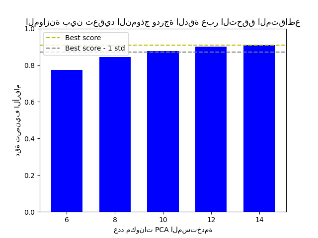
الموازنة بين تعقيد النموذج ودرجة الدقة عبر التحقق المتقاطع

The best_index_ is 2
The n_components selected is 10
The corresponding accuracy score is 0.88

# المؤلفون: مطوري سكايت-ليرن
# معرف الترخيص: BSD-3-Clause

import matplotlib.pyplot as plt
import numpy as np

from sklearn.datasets import load_digits
from sklearn.decomposition import PCA
from sklearn.model_selection import GridSearchCV
from sklearn.pipeline import Pipeline
from sklearn.svm import LinearSVC


def lower_bound(cv_results):
    """
    حساب الحد الأدنى ضمن انحراف معياري واحد
    لأفضل `mean_test_scores`.

    المعاملات
    ----------
    cv_results : dict of numpy(masked) ndarrays
        راجع cv_results_ الخاص بـ `GridSearchCV`

    العائدات
    -------
    float
        الحد الأدنى ضمن انحراف معياري واحد لأفضل
        `mean_test_score`.
    """
    best_score_idx = np.argmax(cv_results["mean_test_score"])

    return (
        cv_results["mean_test_score"][best_score_idx]
        - cv_results["std_test_score"][best_score_idx]
    )


def best_low_complexity(cv_results):
    """
    الموازنة بين تعقيد النموذج ودرجة الدقة عبر التحقق المتقاطع.

    المعاملات
    ----------
    cv_results : dict of numpy(masked) ndarrays
        راجع cv_results_ الخاص بـ `GridSearchCV`.

    العائدات
    ------
    int
        مؤشر نموذج يحتوي على أقل عدد من مكونات PCA
        بينما تكون درجة دقته ضمن انحراف معياري واحد لأفضل
        `mean_test_score`.
    """
    threshold = lower_bound(cv_results)
    candidate_idx = np.flatnonzero(cv_results["mean_test_score"] >= threshold)
    best_idx = candidate_idx[
        cv_results["param_reduce_dim__n_components"][candidate_idx].argmin()
    ]
    return best_idx


pipe = Pipeline(
    [
        ("reduce_dim", PCA(random_state=42)),
        ("classify", LinearSVC(random_state=42, C=0.01)),
    ]
)

param_grid = {"reduce_dim__n_components": [6, 8, 10, 12, 14]}

grid = GridSearchCV(
    pipe,
    cv=10,
    n_jobs=1,
    param_grid=param_grid,
    scoring="accuracy",
    refit=best_low_complexity,
)
X, y = load_digits(return_X_y=True)
grid.fit(X, y)

n_components = grid.cv_results_["param_reduce_dim__n_components"]
test_scores = grid.cv_results_["mean_test_score"]

plt.figure()
plt.bar(n_components, test_scores, width=1.3, color="b")

lower = lower_bound(grid.cv_results_)
plt.axhline(np.max(test_scores), linestyle="--", color="y", label="Best score")
plt.axhline(lower, linestyle="--", color=".5", label="Best score - 1 std")

plt.title("الموازنة بين تعقيد النموذج ودرجة الدقة عبر التحقق المتقاطع")
plt.xlabel("عدد مكونات PCA المستخدمة")
plt.ylabel("دقة تصنيف الأرقام")
plt.xticks(n_components.tolist())
plt.ylim((0, 1.0))
plt.legend(loc="upper left")

best_index_ = grid.best_index_

print("The best_index_ is %d" % best_index_)
print("The n_components selected is %d" % n_components[best_index_])
print(
    "The corresponding accuracy score is %.2f"
    % grid.cv_results_["mean_test_score"][best_index_]
)
plt.show()