ملاحظة

Go to the end to download the full example code. or to run this example in your browser via JupyterLite or Binder

تحليل العوامل (مع الدوران) لتصور الأنماط#

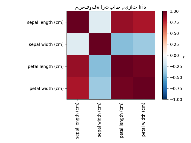
عند دراسة مجموعة بيانات Iris، نلاحظ أن طول السبلة وطول البتلة وعرض البتلة مترابطة بشكل كبير. عرض السبلة أقل تكراراً. يمكن لتقنيات تحليل المصفوفات الكشف عن هذه الأنماط الكامنة. لا يؤدي تطبيق الدوران على المكونات الناتجة إلى تحسين القيمة التنبؤية للمساحة الكامنة المستنبطة بشكل جوهري، ولكن يمكن أن يساعد في تصور بنيتها؛ هنا، على سبيل المثال، يجد دوران Varimax، والذي يتم العثور عليه عن طريق تعظيم التباين التربيعي للأوزان، بنية حيث يحمل المكون الثاني فقط بشكل إيجابي على عرض السبلة.

# المؤلفون: مطوري scikit-learn
# معرف الترخيص: BSD-3-Clause

import matplotlib.pyplot as plt
import numpy as np

from sklearn.datasets import load_iris
from sklearn.decomposition import PCA, FactorAnalysis
from sklearn.preprocessing import StandardScaler

تحميل بيانات Iris

data = load_iris()
X = StandardScaler().fit_transform(data["data"])
feature_names = data["feature_names"]

رسم مصفوفة ارتباط ميزات Iris

ax = plt.axes()

im = ax.imshow(np.corrcoef(X.T), cmap="RdBu_r", vmin=-1, vmax=1)

ax.set_xticks([0, 1, 2, 3])
ax.set_xticklabels(list(feature_names), rotation=90)
ax.set_yticks([0, 1, 2, 3])
ax.set_yticklabels(list(feature_names))

plt.colorbar(im).ax.set_ylabel("$r$", rotation=0)
ax.set_title("مصفوفة ارتباط ميزات Iris")
plt.tight_layout()

تشغيل تحليل العوامل مع دوران Varimax

n_comps = 2

methods = [
    ("PCA", PCA()),
    ("Unrotated FA", FactorAnalysis()),
    ("Varimax FA", FactorAnalysis(rotation="varimax")),
]
fig, axes = plt.subplots(ncols=len(methods), figsize=(10, 8), sharey=True)

for ax, (method, fa) in zip(axes, methods):
    fa.set_params(n_components=n_comps)
    fa.fit(X)

    components = fa.components_.T
    print("\n\n %s :\n" % method)
    print(components)

    vmax = np.abs(components).max()
    ax.imshow(components, cmap="RdBu_r", vmax=vmax, vmin=-vmax)
    ax.set_yticks(np.arange(len(feature_names)))
    ax.set_yticklabels(feature_names)
    ax.set_title(str(method))
    ax.set_xticks([0, 1])
    ax.set_xticklabels(["Comp. 1", "Comp. 2"])
fig.suptitle("Factors")
plt.tight_layout()
plt.show()

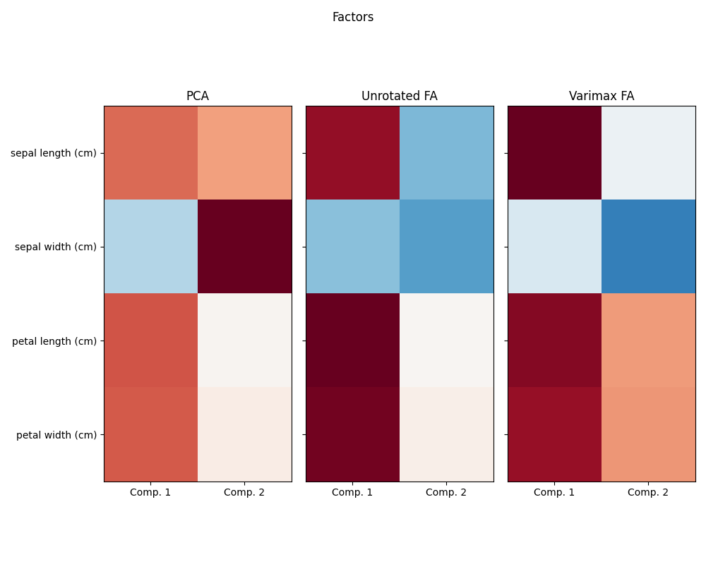
 PCA :

[[ 0.52106591  0.37741762]
 [-0.26934744  0.92329566]
 [ 0.5804131   0.02449161]
 [ 0.56485654  0.06694199]]


 Unrotated FA :

[[ 0.88096009 -0.4472869 ]
 [-0.41691605 -0.55390036]
 [ 0.99918858  0.01915283]
 [ 0.96228895  0.05840206]]


 Varimax FA :

[[ 0.98633022 -0.05752333]
 [-0.16052385 -0.67443065]
 [ 0.90809432  0.41726413]
 [ 0.85857475  0.43847489]]

Total running time of the script: (0 minutes 0.560 seconds)