ملاحظة
Go to the end to download the full example code. or to run this example in your browser via JupyterLite or Binder
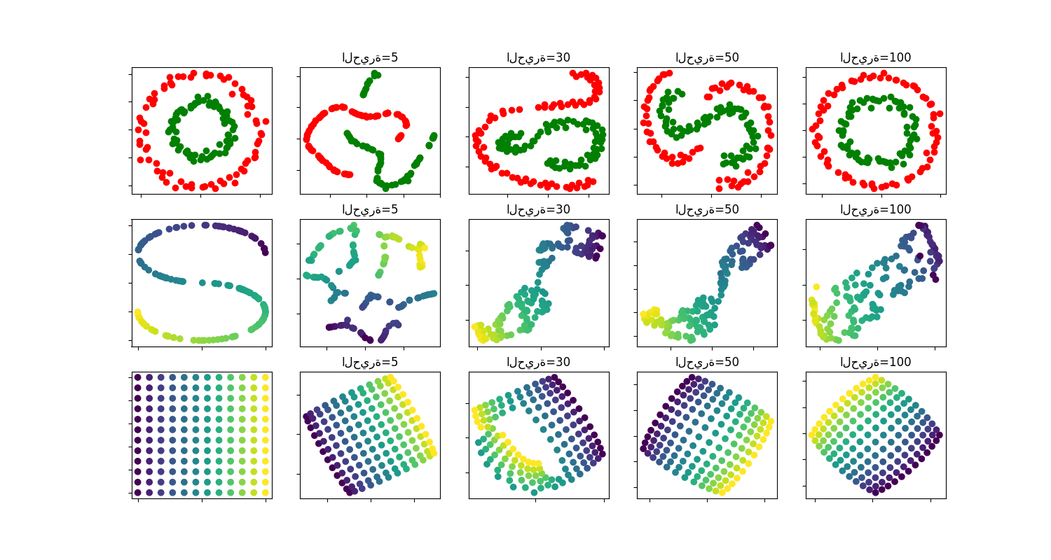
t-SNE: تأثير قيم الحيرة المختلفة على الشكل#
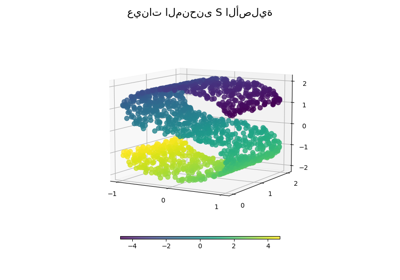
توضيح لـ t-SNE على دائرتين متحدة المركز ومجموعة بيانات المنحنى S لقيم حيرة مختلفة.
نلاحظ ميلًا نحو أشكال أوضح مع زيادة قيمة الحيرة.
قد يختلف حجم ومسافة وشكل المجموعات بناءً على التهيئة وقيم الحيرة ولا ينقل دائمًا معنى.
كما هو موضح أدناه، يجد t-SNE بالنسبة للحيرة الأعلى شكلًا ذا معنى لدائرتين متحدة المركز، ومع ذلك يختلف حجم ومسافة الدوائر قليلاً عن الأصل. على عكس مجموعة بيانات الدائرتين، فإن الأشكال تنحرف بصريًا عن شكل المنحنى S على مجموعة بيانات المنحنى S حتى بالنسبة لقيم الحيرة الأكبر.
لمزيد من التفاصيل، يوفر "كيفية استخدام t-SNE بفعالية" https://distill.pub/2016/misread-tsne/ نقاشًا جيدًا حول تأثيرات المعلمات المختلفة، بالإضافة إلى مخططات تفاعلية لاستكشاف هذه التأثيرات.
الدوائر، الحيرة=5 في 0.14 ثانية
الدوائر، الحيرة=30 في 0.17 ثانية
الدوائر، الحيرة=50 في 0.23 ثانية
الدوائر، الحيرة=100 في 0.19 ثانية
المنحنى S، الحيرة=5 في 0.12 ثانية
المنحنى S، الحيرة=30 في 0.18 ثانية
المنحنى S، الحيرة=50 في 0.17 ثانية
المنحنى S، الحيرة=100 في 0.23 ثانية
الشبكة الموحدة، الحيرة=5 في 0.21 ثانية
الشبكة الموحدة، الحيرة=30 في 0.2 ثانية
الشبكة الموحدة، الحيرة=50 في 0.25 ثانية
الشبكة الموحدة، الحيرة=100 في 0.25 ثانية
# Authors: The scikit-learn developers
# SPDX-License-Identifier: BSD-3-Clause

from time import time

import matplotlib.pyplot as plt
import numpy as np
from matplotlib.ticker import NullFormatter

from sklearn import datasets, manifold

n_samples = 150
n_components = 2
(fig, subplots) = plt.subplots(3, 5, figsize=(15, 8))
perplexities = [5, 30, 50, 100]

X, y = datasets.make_circles(
    n_samples=n_samples, factor=0.5, noise=0.05, random_state=0
)

red = y == 0
green = y == 1

ax = subplots[0][0]
ax.scatter(X[red, 0], X[red, 1], c="r")
ax.scatter(X[green, 0], X[green, 1], c="g")
ax.xaxis.set_major_formatter(NullFormatter())
ax.yaxis.set_major_formatter(NullFormatter())
plt.axis("tight")

for i, perplexity in enumerate(perplexities):
    ax = subplots[0][i + 1]

    t0 = time()
    tsne = manifold.TSNE(
        n_components=n_components,
        init="random",
        random_state=0,
        perplexity=perplexity,
        max_iter=300,
    )
    Y = tsne.fit_transform(X)
    t1 = time()
    print("الدوائر، الحيرة=%d في %.2g ثانية" % (perplexity, t1 - t0))
    ax.set_title("الحيرة=%d" % perplexity)
    ax.scatter(Y[red, 0], Y[red, 1], c="r")
    ax.scatter(Y[green, 0], Y[green, 1], c="g")
    ax.xaxis.set_major_formatter(NullFormatter())
    ax.yaxis.set_major_formatter(NullFormatter())
    ax.axis("tight")

# مثال آخر باستخدام المنحنى S
X, color = datasets.make_s_curve(n_samples, random_state=0)

ax = subplots[1][0]
ax.scatter(X[:, 0], X[:, 2], c=color)
ax.xaxis.set_major_formatter(NullFormatter())
ax.yaxis.set_major_formatter(NullFormatter())

for i, perplexity in enumerate(perplexities):
    ax = subplots[1][i + 1]

    t0 = time()
    tsne = manifold.TSNE(
        n_components=n_components,
        init="random",
        random_state=0,
        perplexity=perplexity,
        learning_rate="auto",
        max_iter=300,
    )
    Y = tsne.fit_transform(X)
    t1 = time()
    print("المنحنى S، الحيرة=%d في %.2g ثانية" % (perplexity, t1 - t0))

    ax.set_title("الحيرة=%d" % perplexity)
    ax.scatter(Y[:, 0], Y[:, 1], c=color)
    ax.xaxis.set_major_formatter(NullFormatter())
    ax.yaxis.set_major_formatter(NullFormatter())
    ax.axis("tight")


# مثال آخر باستخدام شبكة موحدة ثنائية الأبعاد
x = np.linspace(0, 1, int(np.sqrt(n_samples)))
xx, yy = np.meshgrid(x, x)
X = np.hstack(
    [
        xx.ravel().reshape(-1, 1),
        yy.ravel().reshape(-1, 1),
    ]
)
color = xx.ravel()
ax = subplots[2][0]
ax.scatter(X[:, 0], X[:, 1], c=color)
ax.xaxis.set_major_formatter(NullFormatter())
ax.yaxis.set_major_formatter(NullFormatter())

for i, perplexity in enumerate(perplexities):
    ax = subplots[2][i + 1]

    t0 = time()
    tsne = manifold.TSNE(
        n_components=n_components,
        init="random",
        random_state=0,
        perplexity=perplexity,
        max_iter=400,
    )
    Y = tsne.fit_transform(X)
    t1 = time()
    print("الشبكة الموحدة، الحيرة=%d في %.2g ثانية" % (perplexity, t1 - t0))

    ax.set_title("الحيرة=%d" % perplexity)
    ax.scatter(Y[:, 0], Y[:, 1], c=color)
    ax.xaxis.set_major_formatter(NullFormatter())
    ax.yaxis.set_major_formatter(NullFormatter())
    ax.axis("tight")


plt.show()
Total running time of the script: (0 minutes 3.296 seconds)
Related examples
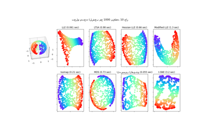

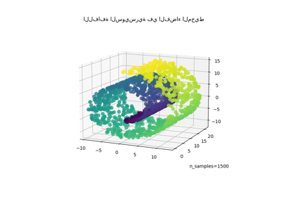
خفض اللفافة السويسرية واللفافة السويسرية ذات الثقب