ملاحظة
Go to the end to download the full example code. or to run this example in your browser via JupyterLite or Binder
طرق تعلم متعدد الشعب على كرة مقطوعة#
تطبيق مختلف تقنيات متعدد الشعب على مجموعة بيانات كروية. هنا يمكن للمرء أن يرى استخدام خفض الأبعاد من أجل اكتساب بعض الحدس بخصوص طرق تعلم متعدد الشعب. فيما يتعلق بمجموعة البيانات، يتم قطع القطبين من الكرة، بالإضافة إلى شريحة رقيقة على جانبها. هذا يتيح لتقنيات تعلم متعدد الشعب "فردها" أثناء إسقاطها على بُعدين.
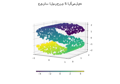
لمثال مماثل، حيث يتم تطبيق الطرق على مجموعة بيانات المنحنى S، انظر مقارنة طرق تعلم متعدد الشعب
لاحظ أن الغرض من MDS هو إيجاد تمثيل منخفض الأبعاد للبيانات (هنا 2D) فيه المسافات تحترم جيدًا المسافات في الفضاء الأصلي عالي الأبعاد، على عكس خوارزميات تعلم متعدد الشعب الأخرى، فهي لا تسعى إلى تمثيل متماثل للبيانات في الفضاء منخفض الأبعاد. هنا تتطابق مشكلة متعدد الشعب بشكل كبير مع تمثيل خريطة مسطحة للأرض، كما هو الحال مع إسقاط الخريطة
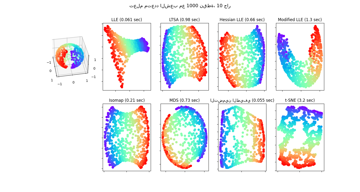
standard: 0.061 sec
ltsa: 0.98 sec
hessian: 0.66 sec
modified: 1.3 sec
ISO: 0.21 sec
MDS: 0.73 sec
Spectral Embedding: 0.055 sec
t-SNE: 3.2 sec
# Authors: The scikit-learn developers
# SPDX-License-Identifier: BSD-3-Clause

from time import time

import matplotlib.pyplot as plt

# Unused but required import for doing 3d projections with matplotlib < 3.2
import mpl_toolkits.mplot3d  # noqa: F401
import numpy as np
from matplotlib.ticker import NullFormatter

from sklearn import manifold
from sklearn.utils import check_random_state

# متغيرات لتعلم متعدد الشعب.
n_neighbors = 10
n_samples = 1000

# إنشاء الكرة.
random_state = check_random_state(0)
p = random_state.rand(n_samples) * (2 * np.pi - 0.55)
t = random_state.rand(n_samples) * np.pi

# قطع القطبين من الكرة.
indices = (t < (np.pi - (np.pi / 8))) & (t > ((np.pi / 8)))
colors = p[indices]
x, y, z = (
    np.sin(t[indices]) * np.cos(p[indices]),
    np.sin(t[indices]) * np.sin(p[indices]),
    np.cos(t[indices]),
)

# رسم مجموعة البيانات.
fig = plt.figure(figsize=(15, 8))
plt.suptitle(
    "تعلم متعدد الشعب مع %i نقطة، %i جار" % (1000, n_neighbors), fontsize=14
)

ax = fig.add_subplot(251, projection="3d")
ax.scatter(x, y, z, c=p[indices], cmap=plt.cm.rainbow)
ax.view_init(40, -10)

sphere_data = np.array([x, y, z]).T

# إجراء تعلم متعدد الشعب بالتضمين الخطي المحلي
methods = ["standard", "ltsa", "hessian", "modified"]
labels = ["LLE", "LTSA", "Hessian LLE", "Modified LLE"]

for i, method in enumerate(methods):
    t0 = time()
    trans_data = (
        manifold.LocallyLinearEmbedding(
            n_neighbors=n_neighbors, n_components=2, method=method, random_state=42
        )
        .fit_transform(sphere_data)
        .T
    )
    t1 = time()
    print("%s: %.2g sec" % (methods[i], t1 - t0))

    ax = fig.add_subplot(252 + i)
    plt.scatter(trans_data[0], trans_data[1], c=colors, cmap=plt.cm.rainbow)
    plt.title("%s (%.2g sec)" % (labels[i], t1 - t0))
    ax.xaxis.set_major_formatter(NullFormatter())
    ax.yaxis.set_major_formatter(NullFormatter())
    plt.axis("tight")

# إجراء تعلم متعدد الشعب باستخدام Isomap.
t0 = time()
trans_data = (
    manifold.Isomap(n_neighbors=n_neighbors, n_components=2)
    .fit_transform(sphere_data)
    .T
)
t1 = time()
print("%s: %.2g sec" % ("ISO", t1 - t0))

ax = fig.add_subplot(257)
plt.scatter(trans_data[0], trans_data[1], c=colors, cmap=plt.cm.rainbow)
plt.title("%s (%.2g sec)" % ("Isomap", t1 - t0))
ax.xaxis.set_major_formatter(NullFormatter())
ax.yaxis.set_major_formatter(NullFormatter())
plt.axis("tight")

# إجراء القياس متعدد الأبعاد.
t0 = time()
mds = manifold.MDS(2, max_iter=100, n_init=1, random_state=42)
trans_data = mds.fit_transform(sphere_data).T
t1 = time()
print("MDS: %.2g sec" % (t1 - t0))

ax = fig.add_subplot(258)
plt.scatter(trans_data[0], trans_data[1], c=colors, cmap=plt.cm.rainbow)
plt.title("MDS (%.2g sec)" % (t1 - t0))
ax.xaxis.set_major_formatter(NullFormatter())
ax.yaxis.set_major_formatter(NullFormatter())
plt.axis("tight")

# إجراء التضمين الطيفي.
t0 = time()
se = manifold.SpectralEmbedding(
    n_components=2, n_neighbors=n_neighbors, random_state=42
)
trans_data = se.fit_transform(sphere_data).T
t1 = time()
print("Spectral Embedding: %.2g sec" % (t1 - t0))

ax = fig.add_subplot(259)
plt.scatter(trans_data[0], trans_data[1], c=colors, cmap=plt.cm.rainbow)
plt.title("التضمين الطيفي (%.2g sec)" % (t1 - t0))
ax.xaxis.set_major_formatter(NullFormatter())
ax.yaxis.set_major_formatter(NullFormatter())
plt.axis("tight")

# إجراء تضمين الجوار العشوائي الموزع على شكل حرف t.
t0 = time()
tsne = manifold.TSNE(n_components=2, random_state=0)
trans_data = tsne.fit_transform(sphere_data).T
t1 = time()
print("t-SNE: %.2g sec" % (t1 - t0))

ax = fig.add_subplot(2, 5, 10)
plt.scatter(trans_data[0], trans_data[1], c=colors, cmap=plt.cm.rainbow)
plt.title("t-SNE (%.2g sec)" % (t1 - t0))
ax.xaxis.set_major_formatter(NullFormatter())
ax.yaxis.set_major_formatter(NullFormatter())
plt.axis("tight")

plt.show()
Total running time of the script: (0 minutes 8.049 seconds)
Related examples
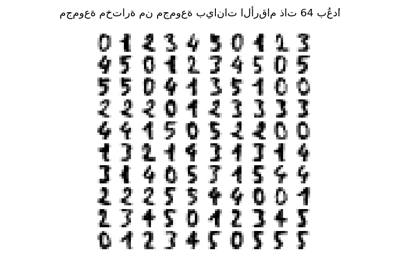
تعلم متعدد الشعب على الأرقام المكتوبة بخط اليد: التضمين الخطي المحلي، Isomap...