ملاحظة
Go to the end to download the full example code. or to run this example in your browser via JupyterLite or Binder
تطبيق خوارزمية k-means على مجموعة البيانات digits#
هذا المثال يهدف إلى توضيح المواقف التي تنتج فيها خوارزمية كاي-مينز (k-means) تجميعات غير بديهية وربما غير مرغوب فيها.
# المؤلفون: مطوّرو سكايلرن (scikit-learn)
# معرف رخصة SPDX: BSD-3-Clause
تحميل مجموعة البيانات#
سنبدأ بتحميل مجموعة بيانات digits. تحتوي هذه المجموعة على
أرقام مكتوبة بخط اليد من 0 إلى 9. في سياق التجميع، يرغب المرء
في تجميع الصور بحيث تكون الأرقام المكتوبة بخط اليد على الصورة متطابقة.
import numpy as np

from sklearn.datasets import load_digits

data, labels = load_digits(return_X_y=True)
(n_samples, n_features), n_digits = data.shape, np.unique(labels).size

print(f"# digits: {n_digits}; # samples: {n_samples}; # features {n_features}")
# digits: 10; # samples: 1797; # features 64
تحديد معيار التقييم الخاص بنا#
سنقوم أولاً بتحديد معيار التقييم الخاص بنا. خلال هذا المعيار، نعتزم مقارنة طرق التهيئة المختلفة لـ KMeans. سيتضمن معيارنا:
إنشاء خط أنابيب سيقوم بتصعيد البيانات باستخدام
StandardScaler؛تدريب وتوقيت ملاءمة خط الأنابيب؛
قياس أداء التجميع الذي تم الحصول عليه عبر مقاييس مختلفة.
from time import time

from sklearn import metrics
from sklearn.pipeline import make_pipeline
from sklearn.preprocessing import StandardScaler


def bench_k_means(kmeans, name, data, labels):
    """معيار لتقييم طرق تهيئة KMeans.

    Parameters
    ----------
    kmeans : KMeans instance
        A :class:`~sklearn.cluster.KMeans` instance with the initialization
        already set.
    name : str
        Name given to the strategy. It will be used to show the results in a
        table.
    data : ndarray of shape (n_samples, n_features)
        The data to cluster.
    labels : ndarray of shape (n_samples,)
        The labels used to compute the clustering metrics which requires some
        supervision.
    """
    t0 = time()
    estimator = make_pipeline(StandardScaler(), kmeans).fit(data)
    fit_time = time() - t0
    results = [name, fit_time, estimator[-1].inertia_]

    # Define the metrics which require only the true labels and estimator
    # labels
    clustering_metrics = [
        metrics.homogeneity_score,
        metrics.completeness_score,
        metrics.v_measure_score,
        metrics.adjusted_rand_score,
        metrics.adjusted_mutual_info_score,
    ]
    results += [m(labels, estimator[-1].labels_) for m in clustering_metrics]

    # The silhouette score requires the full dataset
    results += [
        metrics.silhouette_score(
            data,
            estimator[-1].labels_,
            metric="euclidean",
            sample_size=300,
        )
    ]

    # Show the results
    formatter_result = (
        "{:9s}\t{:.3f}s\t{:.0f}\t{:.3f}\t{:.3f}\t{:.3f}\t{:.3f}\t{:.3f}\t{:.3f}"
    )
    print(formatter_result.format(*results))
# Show the results
    formatter_result = (
        "{:9s}\t{:.3f}s\t{:.0f}\t{:.3f}\t{:.3f}\t{:.3f}\t{:.3f}\t{:.3f}\t{:.3f}"
    )
    print(formatter_result.format(*results))
تشغيل المعيار#
سنقارن بين ثلاثة نهج:
تهيئة باستخدام
k-means++. هذه الطريقة عشوائية وسنقوم بتشغيل التهيئة 4 مرات؛تهيئة عشوائية. هذه الطريقة عشوائية أيضًا وسنقوم بتشغيل التهيئة 4 مرات؛
تهيئة تعتمد على
PCAالإسقاط. في الواقع، سنستخدم مكوناتPCAلتهيئة KMeans. هذه الطريقة حتمية وتكفي عملية تهيئة واحدة.
from sklearn.cluster import KMeans
from sklearn.decomposition import PCA

print(82 * "_")
print("init\t\ttime\tinertia\thomo\tcompl\tv-meas\tARI\tAMI\tsilhouette")

kmeans = KMeans(init="k-means++", n_clusters=n_digits, n_init=4, random_state=0)
bench_k_means(kmeans=kmeans, name="k-means++", data=data, labels=labels)

kmeans = KMeans(init="random", n_clusters=n_digits, n_init=4, random_state=0)
bench_k_means(kmeans=kmeans, name="random", data=data, labels=labels)

pca = PCA(n_components=n_digits).fit(data)
kmeans = KMeans(init=pca.components_, n_clusters=n_digits, n_init=1)
bench_k_means(kmeans=kmeans, name="PCA-based", data=data, labels=labels)

print(82 * "_")
__________________________________________________________________________________
init            time    inertia homo    compl   v-meas  ARI     AMI     silhouette
k-means++       0.028s  69545   0.598   0.645   0.621   0.469   0.617   0.169
k-means++       0.028s  69545   0.598   0.645   0.621   0.469   0.617   0.169
random          0.108s  69735   0.681   0.723   0.701   0.574   0.698   0.182
random          0.108s  69735   0.681   0.723   0.701   0.574   0.698   0.182
PCA-based       0.115s  69513   0.600   0.647   0.622   0.468   0.618   0.140
PCA-based       0.115s  69513   0.600   0.647   0.622   0.468   0.618   0.140
__________________________________________________________________________________
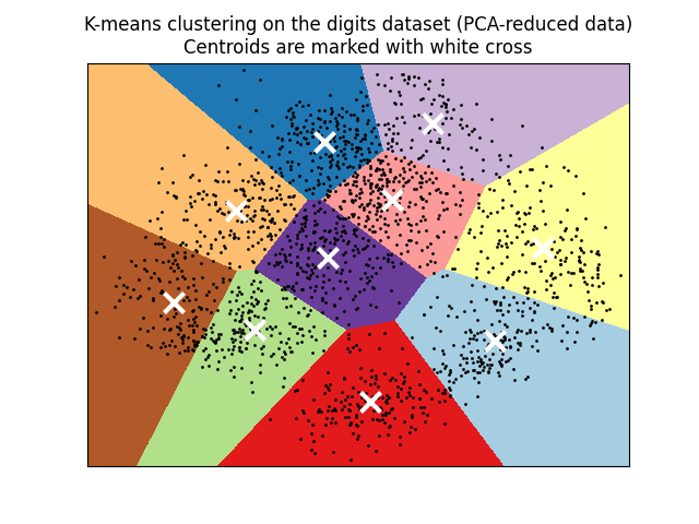
تصور النتائج على البيانات المخفضة بواسطة PCA#
PCA يسمح بتصوير البيانات من
المساحة الأصلية ذات 64 بُعدًا إلى مساحة ذات أبعاد أقل. بعد ذلك،
يمكننا استخدام PCA لتصويرها في
مساحة ثنائية الأبعاد ورسم البيانات والمجموعات في هذه المساحة الجديدة.
import matplotlib.pyplot as plt

reduced_data = PCA(n_components=2).fit_transform(data)
kmeans = KMeans(init="k-means++", n_clusters=n_digits, n_init=4)
kmeans.fit(reduced_data)

# حجم خط الشبكة. قلل لتحسين جودة VQ.
h = 0.02  # point in the mesh [x_min, x_max]x[y_min, y_max].

# Plot the decision boundary. For that, we will assign a color to each
x_min, x_max = reduced_data[:, 0].min() - 1, reduced_data[:, 0].max() + 1
y_min, y_max = reduced_data[:, 1].min() - 1, reduced_data[:, 1].max() + 1
xx, yy = np.meshgrid(np.arange(x_min, x_max, h), np.arange(y_min, y_max, h))

# Obtain labels for each point in mesh. Use last trained model.
Z = kmeans.predict(np.c_[xx.ravel(), yy.ravel()])

# Put the result into a color plot
Z = Z.reshape(xx.shape)
plt.figure(1)
plt.clf()
plt.imshow(
    Z,
    interpolation="nearest",
    extent=(xx.min(), xx.max(), yy.min(), yy.max()),
    cmap=plt.cm.Paired,
    aspect="auto",
    origin="lower",
)

plt.plot(reduced_data[:, 0], reduced_data[:, 1], "k.", markersize=2)
# Plot the centroids as a white X
centroids = kmeans.cluster_centers_
plt.scatter(
    centroids[:, 0],
    centroids[:, 1],
    marker="x",
    s=169,
    linewidths=3,
    color="w",
    zorder=10,
)
plt.title(
    "K-means clustering on the digits dataset (PCA-reduced data)\n"
    "Centroids are marked with white cross"
)
plt.xlim(x_min, x_max)
plt.ylim(y_min, y_max)
plt.xticks(())
plt.yticks(())
plt.show()
Total running time of the script: (0 minutes 1.096 seconds)
Related examples
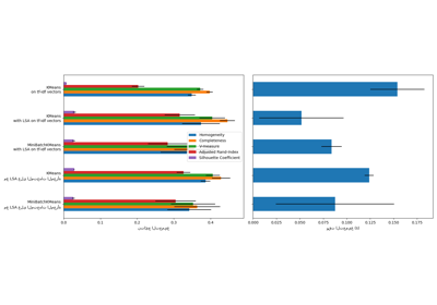
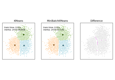
مقارنة خوارزميات التجميع K-Means و MiniBatchKMeans
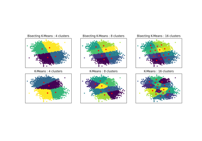
sphx_glr_auto_examples_cluster_plot_bisect_kmeans.py