ملاحظة

Go to the end to download the full example code. or to run this example in your browser via JupyterLite or Binder

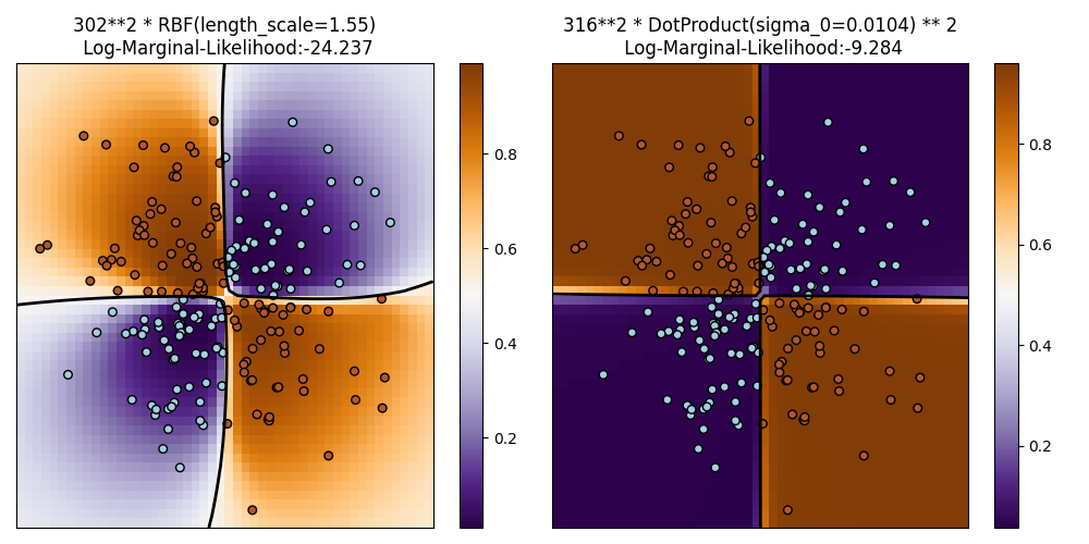
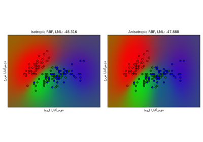
توضيح تصنيف العملية الغاوسية (GPC) على مجموعة بيانات XOR#

يوضح هذا المثال GPC على بيانات XOR. تتم مقارنة نواة ثابتة ومتناحرة (RBF) بنواة غير ثابتة (DotProduct). في مجموعة البيانات هذه تحديدًا ، تحصل نواة DotProduct على نتائج أفضل بكثير لأن حدود الفئة خطية وتتوافق مع محاور الإحداثيات. بشكل عام ، غالبًا ما تحقق النوى الثابتة نتائج أفضل.

302**2 * RBF(length_scale=1.55) Log-Marginal-Likelihood:-24.237, 316**2 * DotProduct(sigma_0=0.0104) ** 2 Log-Marginal-Likelihood:-9.284

/project/workspace/sklearn/gaussian_process/kernels.py:452: ConvergenceWarning:

The optimal value found for dimension 0 of parameter k1__constant_value is close to the specified upper bound 100000.0. Increasing the bound and calling fit again may find a better value.

# Authors: The scikit-learn developers
# SPDX-License-Identifier: BSD-3-Clause

import matplotlib.pyplot as plt
import numpy as np

from sklearn.gaussian_process import GaussianProcessClassifier
from sklearn.gaussian_process.kernels import RBF, DotProduct

xx, yy = np.meshgrid(np.linspace(-3, 3, 50), np.linspace(-3, 3, 50))
rng = np.random.RandomState(0)
X = rng.randn(200, 2)
Y = np.logical_xor(X[:, 0] > 0, X[:, 1] > 0)

# ملاءمة النموذج
plt.figure(figsize=(10, 5))
kernels = [1.0 * RBF(length_scale=1.15), 1.0 * DotProduct(sigma_0=1.0) ** 2]
for i, kernel in enumerate(kernels):
    clf = GaussianProcessClassifier(kernel=kernel, warm_start=True).fit(X, Y)

    # رسم دالة القرار لكل نقطة بيانات على الشبكة
    Z = clf.predict_proba(np.vstack((xx.ravel(), yy.ravel())).T)[:, 1]
    Z = Z.reshape(xx.shape)

    plt.subplot(1, 2, i + 1)
    image = plt.imshow(
        Z,
        interpolation="nearest",
        extent=(xx.min(), xx.max(), yy.min(), yy.max()),
        aspect="auto",
        origin="lower",
        cmap=plt.cm.PuOr_r,
    )
    contours = plt.contour(xx, yy, Z, levels=[0.5], linewidths=2, colors=["k"])
    plt.scatter(X[:, 0], X[:, 1], s=30, c=Y, cmap=plt.cm.Paired, edgecolors=(0, 0, 0))
    plt.xticks(())
    plt.yticks(())
    plt.axis([-3, 3, -3, 3])
    plt.colorbar(image)
    plt.title(
        "%s\n Log-Marginal-Likelihood:%.3f"
        % (clf.kernel_, clf.log_marginal_likelihood(clf.kernel_.theta)),
        fontsize=12,
    )

plt.tight_layout()
plt.show()