ملاحظة

Go to the end to download the full example code. or to run this example in your browser via JupyterLite or Binder

الاختيار المشترك للميزات باستخدام Lasso متعدد المهام#

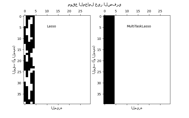
يسمح Lasso متعدد المهام بتناسب مشاكل الانحدار المتعددة فرض اختيار الميزات نفسها عبر المهام. يحاكي هذا المثال القياسات التسلسلية، حيث تمثل كل مهمة لحظة زمنية، وتختلف الميزات ذات الصلة في السعة بمرور الوقت مع بقائها نفسها. يفرض Lasso متعدد المهام أن الميزات التي يتم اختيارها في لحظة زمنية واحدة يتم اختيارها لجميع اللحظات الزمنية. وهذا يجعل اختيار الميزات بواسطة Lasso أكثر استقرارًا.

# المؤلفون: مطوري scikit-learn
# معرف الترخيص: BSD-3-Clause

توليد البيانات#

import numpy as np

rng = np.random.RandomState(42)

# توليد بعض معاملات ثنائية الأبعاد مع موجات الجيب ذات التردد العشوائي والطور
n_samples, n_features, n_tasks = 100, 30, 40
n_relevant_features = 5
coef = np.zeros((n_tasks, n_features))
times = np.linspace(0, 2 * np.pi, n_tasks)
for k in range(n_relevant_features):
    coef[:, k] = np.sin((1.0 + rng.randn(1)) * times + 3 * rng.randn(1))

X = rng.randn(n_samples, n_features)
Y = np.dot(X, coef.T) + rng.randn(n_samples, n_tasks)

ملاءمة النماذج#

from sklearn.linear_model import Lasso, MultiTaskLasso

coef_lasso_ = np.array([Lasso(alpha=0.5).fit(X, y).coef_ for y in Y.T])
coef_multi_task_lasso_ = MultiTaskLasso(alpha=1.0).fit(X, Y).coef_

رسم الدعم والسلاسل الزمنية#

import matplotlib.pyplot as plt

fig = plt.figure(figsize=(8, 5))
plt.subplot(1, 2, 1)
plt.spy(coef_lasso_)
plt.xlabel("الميزة")
plt.ylabel("الوقت (أو المهمة)")
plt.text(10, 5, "Lasso")
plt.subplot(1, 2, 2)
plt.spy(coef_multi_task_lasso_)
plt.xlabel("الميزة")
plt.ylabel("الوقت (أو المهمة)")
plt.text(10, 5, "MultiTaskLasso")
fig.suptitle("موقع المعامل غير الصفري")

feature_to_plot = 0
plt.figure()
lw = 2
plt.plot(coef[:, feature_to_plot], color="seagreen", linewidth=lw, label="الحقيقة الأرضية")
plt.plot(
    coef_lasso_[:, feature_to_plot], color="cornflowerblue", linewidth=lw, label="Lasso"
)
plt.plot(
    coef_multi_task_lasso_[:, feature_to_plot],
    color="gold",
    linewidth=lw,
    label="MultiTaskLasso",
)
plt.legend(loc="upper center")
plt.axis("tight")
plt.ylim([-1.1, 1.1])
plt.show()