ملاحظة
Go to the end to download the full example code. or to run this example in your browser via JupyterLite or Binder
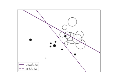
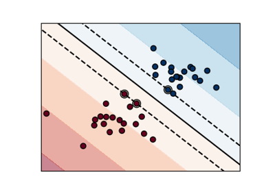
تمرين SVM#
تمرين تعليمي لاستخدام نوى SVM المختلفة.
يتم استخدام هذا التمرين في جزء using_kernels_tut من قسم supervised_learning_tut من stat_learn_tut_index.
# Authors: The scikit-learn developers
# SPDX-License-Identifier: BSD-3-Clause
import matplotlib.pyplot as plt
import numpy as np
from sklearn import datasets, svm
iris = datasets.load_iris()
X = iris.data
y = iris.target
X = X[y != 0, :2]
y = y[y != 0]
n_sample = len(X)
np.random.seed(0)
order = np.random.permutation(n_sample)
X = X[order]
y = y[order].astype(float)
X_train = X[: int(0.9 * n_sample)]
y_train = y[: int(0.9 * n_sample)]
X_test = X[int(0.9 * n_sample):]
y_test = y[int(0.9 * n_sample):]
# ملاءمة النموذج
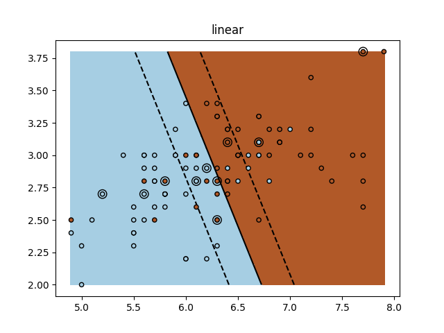
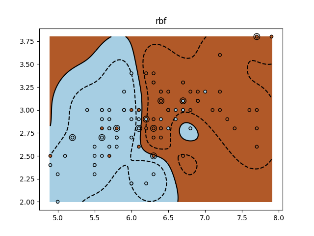
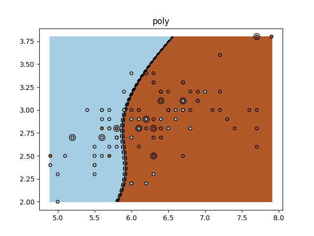
for kernel in ("linear", "rbf", "poly"):
clf = svm.SVC(kernel=kernel, gamma=10)
clf.fit(X_train, y_train)
plt.figure()
plt.clf()
plt.scatter(
X[:, 0], X[:, 1], c=y, zorder=10, cmap=plt.cm.Paired, edgecolor="k", s=20
)
# ضع دائرة حول بيانات الاختبار
plt.scatter(
X_test[:, 0], X_test[:, 1], s=80, facecolors="none", zorder=10, edgecolor="k"
)
plt.axis("tight")
x_min = X[:, 0].min()
x_max = X[:, 0].max()
y_min = X[:, 1].min()
y_max = X[:, 1].max()
XX, YY = np.mgrid[x_min:x_max:200j, y_min:y_max:200j]
Z = clf.decision_function(np.c_[XX.ravel(), YY.ravel()])
# ضع النتيجة في مخطط ألوان
Z = Z.reshape(XX.shape)
plt.pcolormesh(XX, YY, Z > 0, cmap=plt.cm.Paired)
plt.contour(
XX,
YY,
Z,
colors=["k", "k", "k"],
linestyles=["--", "-", "--"],
levels=[-0.5, 0, 0.5],
)
plt.title(kernel)
plt.show()
Total running time of the script: (0 minutes 5.811 seconds)
Related examples
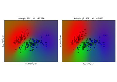
تصنيف العملية الغاوسية (GPC) على مجموعة بيانات iris
تصنيف العملية الغاوسية (GPC) على مجموعة بيانات iris
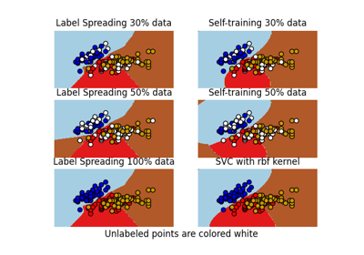
حدود القرار للمصنفات شبه المُشرفة مقابل SVM على مجموعة بيانات Iris
حدود القرار للمصنفات شبه المُشرفة مقابل SVM على مجموعة بيانات Iris