ملاحظة
Go to the end to download the full example code. or to run this example in your browser via JupyterLite or Binder
مقارنة طرق التحليل التفاضلي#
الاستخدام البسيط لخوارزميات التحليل التفاضلي المختلفة:
PLSCanonical
PLSRegression، مع استجابة متعددة المتغيرات، المعروف أيضًا باسم PLS2
PLSRegression، مع استجابة أحادية المتغير، المعروف أيضًا باسم PLS1
CCA
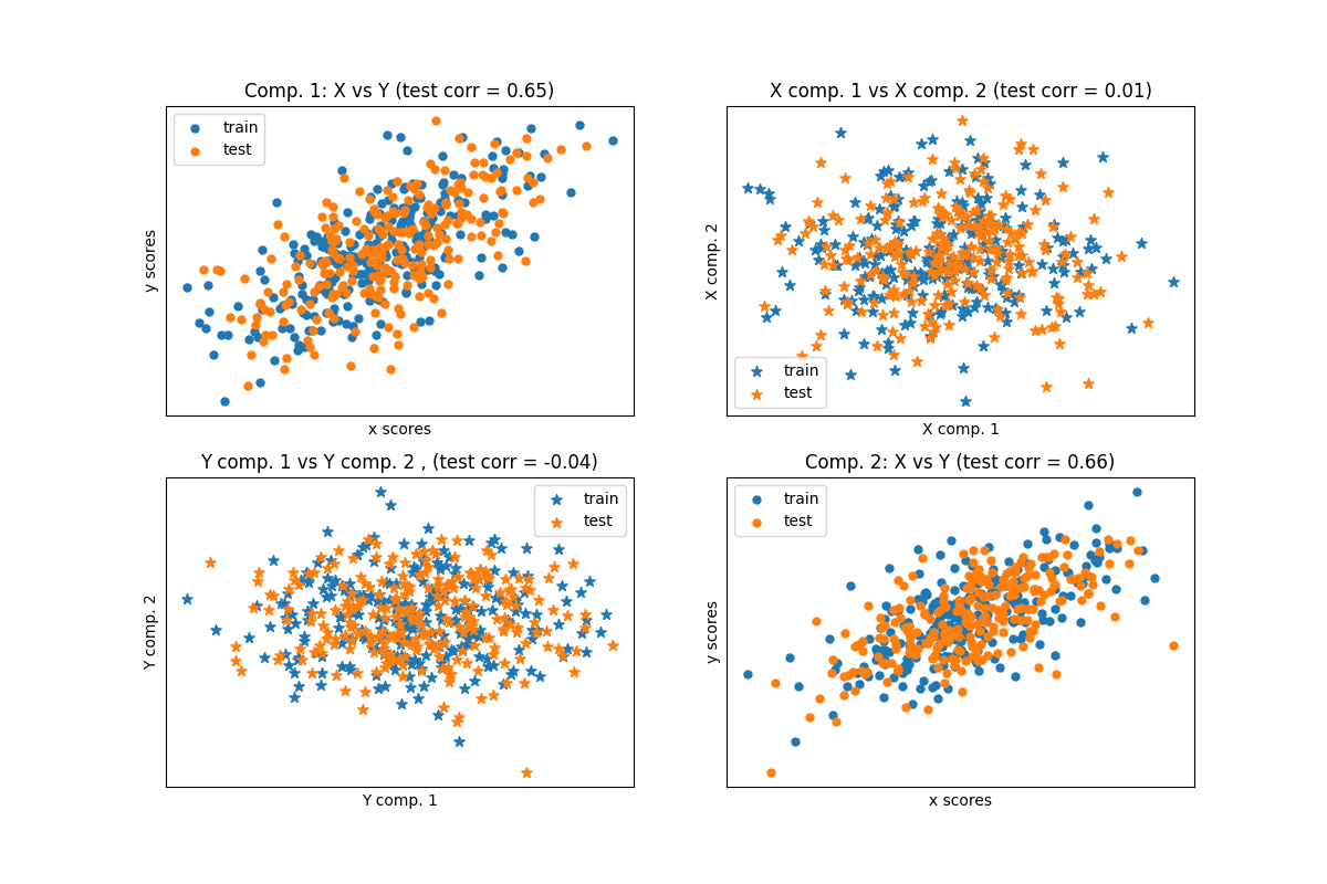
نظرًا لوجود مجموعتين من البيانات ثنائية الأبعاد متعددة المتغيرات ومتغيرة التغاير، X و Y، يقوم PLS باستخراج 'اتجاهات التغاير'، أي مكونات كل مجموعات البيانات التي تفسر أكبر تغاير مشترك بين مجموعتي البيانات. هذا واضح على عرض مصفوفة الرسم البياني: المكونات 1 في مجموعة البيانات X ومجموعة البيانات Y متوافقة بشكل كبير (تتركز النقاط حول المحور الأول). هذا صحيح أيضًا للمكونات 2 في كلتا مجموعتي البيانات، ومع ذلك، فإن الارتباط عبر مجموعات البيانات لمكونات مختلفة ضعيف: سحابة النقاط كروية جدًا.
# المؤلفون: مطوري scikit-learn
# معرف الترخيص: BSD-3-Clause
نموذج المتغيرات الكامنة القائم على مجموعة البيانات#
import numpy as np

n = 500
# 2 متغيرات كامنة:
l1 = np.random.normal(size=n)
l2 = np.random.normal(size=n)

latents = np.array([l1, l1, l2, l2]).T
X = latents + np.random.normal(size=4 * n).reshape((n, 4))
Y = latents + np.random.normal(size=4 * n).reshape((n, 4))

X_train = X[: n // 2]
Y_train = Y[: n // 2]
X_test = X[n // 2 :]
Y_test = Y[n // 2 :]

print("Corr(X)")
print(np.round(np.corrcoef(X.T), 2))
print("Corr(Y)")
print(np.round(np.corrcoef(Y.T), 2))
Corr(X)
[[ 1.    0.49 -0.   -0.07]
 [ 0.49  1.    0.   -0.05]
 [-0.    0.    1.    0.49]
 [-0.07 -0.05  0.49  1.  ]]
Corr(Y)
[[ 1.    0.54  0.02  0.02]
 [ 0.54  1.   -0.05  0.02]
 [ 0.02 -0.05  1.    0.5 ]
 [ 0.02  0.02  0.5   1.  ]]
PLS التطابق (المتماثل)#
تحويل البيانات#
from sklearn.cross_decomposition import PLSCanonical

plsca = PLSCanonical(n_components=2)
plsca.fit(X_train, Y_train)
X_train_r, Y_train_r = plsca.transform(X_train, Y_train)
X_test_r, Y_test_r = plsca.transform(X_test, Y_test)
رسم بياني متفرق لدرجات المكونات#
import matplotlib.pyplot as plt

# على رسم بياني قطري X مقابل Y على كل مكون
plt.figure(figsize=(12, 8))
plt.subplot(221)
plt.scatter(X_train_r[:, 0], Y_train_r[:, 0], label="train", marker="o", s=25)
plt.scatter(X_test_r[:, 0], Y_test_r[:, 0], label="test", marker="o", s=25)
plt.xlabel("x scores")
plt.ylabel("y scores")
plt.title(
    "Comp. 1: X vs Y (test corr = %.2f)"
    % np.corrcoef(X_test_r[:, 0], Y_test_r[:, 0])[0, 1]
)
plt.xticks(())
plt.yticks(())
plt.legend(loc="best")

plt.subplot(224)
plt.scatter(X_train_r[:, 1], Y_train_r[:, 1], label="train", marker="o", s=25)
plt.scatter(X_test_r[:, 1], Y_test_r[:, 1], label="test", marker="o", s=25)
plt.xlabel("x scores")
plt.ylabel("y scores")
plt.title(
    "Comp. 2: X vs Y (test corr = %.2f)"
    % np.corrcoef(X_test_r[:, 1], Y_test_r[:, 1])[0, 1]
)
plt.xticks(())
plt.yticks(())
plt.legend(loc="best")

# رسم بياني خارجي للمكونات 1 مقابل 2 لـ X و Y
plt.subplot(222)
plt.scatter(X_train_r[:, 0], X_train_r[:, 1], label="train", marker="*", s=50)
plt.scatter(X_test_r[:, 0], X_test_r[:, 1], label="test", marker="*", s=50)
plt.xlabel("X comp. 1")
plt.ylabel("X comp. 2")
plt.title(
    "X comp. 1 vs X comp. 2 (test corr = %.2f)"
    % np.corrcoef(X_test_r[:, 0], X_test_r[:, 1])[0, 1]
)
plt.legend(loc="best")
plt.xticks(())
plt.yticks(())

plt.subplot(223)
plt.scatter(Y_train_r[:, 0], Y_train_r[:, 1], label="train", marker="*", s=50)
plt.scatter(Y_test_r[:, 0], Y_test_r[:, 1], label="test", marker="*", s=50)
plt.xlabel("Y comp. 1")
plt.ylabel("Y comp. 2")
plt.title(
    "Y comp. 1 vs Y comp. 2 , (test corr = %.2f)"
    % np.corrcoef(Y_test_r[:, 0], Y_test_r[:, 1])[0, 1]
)
plt.legend(loc="best")
plt.xticks(())
plt.yticks(())
plt.show()
الانحدار PLS، مع استجابة متعددة المتغيرات، المعروف أيضًا باسم PLS2#
from sklearn.cross_decomposition import PLSRegression

n = 1000
q = 3
p = 10
X = np.random.normal(size=n * p).reshape((n, p))
B = np.array([[1, 2] + [0] * (p - 2)] * q).T
# كل Yj = 1*X1 + 2*X2 + ضجيج
Y = np.dot(X, B) + np.random.normal(size=n * q).reshape((n, q)) + 5
pls2 = PLSRegression(n_components=3)
pls2.fit(X, Y)
print("True B (such that: Y = XB + Err)")
print(B)
# compare pls2.coef_ with B
print("Estimated B")
print(np.round(pls2.coef_, 1))
pls2.predict(X)
True B (such that: Y = XB + Err)
[[1 1 1]
 [2 2 2]
 [0 0 0]
 [0 0 0]
 [0 0 0]
 [0 0 0]
 [0 0 0]
 [0 0 0]
 [0 0 0]
 [0 0 0]]
Estimated B
[[ 1.   2.   0.   0.  -0.1 -0.  -0.  -0.1  0.1  0.1]
 [ 1.   2.  -0.  -0.   0.  -0.  -0.   0.  -0.  -0. ]
 [ 1.   2.  -0.  -0.   0.  -0.  -0.   0.  -0.  -0. ]]

array([[5.24380887, 4.90011096, 4.91029934],
       [8.54677264, 8.61106858, 8.57593744],
       [7.20561962, 7.50134877, 7.44172352],
       ...,
       [6.39207502, 6.41414291, 6.38492145],
       [5.76242479, 5.54081118, 5.53736656],
       [3.83619039, 3.55199171, 3.55603776]])
الانحدار PLS، مع استجابة أحادية المتغير، المعروف أيضًا باسم PLS1#
n = 1000
p = 10
X = np.random.normal(size=n * p).reshape((n, p))
y = X[:, 0] + 2 * X[:, 1] + np.random.normal(size=n * 1) + 5
pls1 = PLSRegression(n_components=3)
pls1.fit(X, y)
# لاحظ أن عدد المكونات يتجاوز 1 (بعد y)
print("Estimated betas")
print(np.round(pls1.coef_, 1))
Estimated betas
[[ 1.   2.  -0.1 -0.  -0.  -0.   0.   0.  -0.   0. ]]
CCA (وضع PLS B مع الانكماش المتماثل)#
Total running time of the script: (0 minutes 0.221 seconds)
Related examples
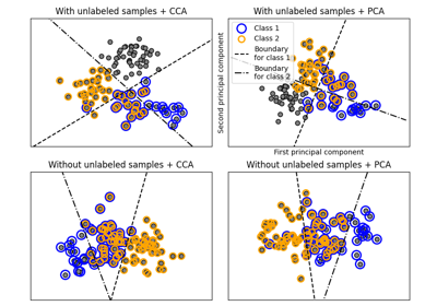
الانحدار باستخدام المكونات الرئيسية مقابل الانحدار باستخدام المربعات الجزئية