ملاحظة
Go to the end to download the full example code. or to run this example in your browser via JupyterLite or Binder
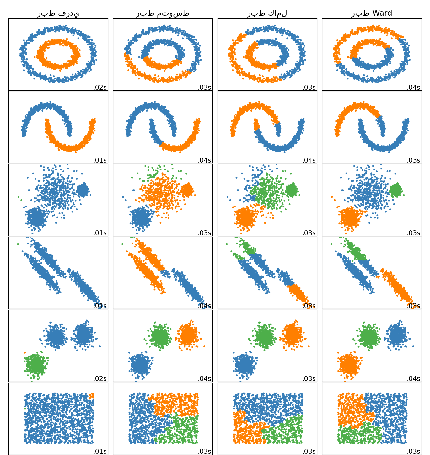
مقارنة طرق الربط الهرمي المختلفة على مجموعات بيانات تجريبية#
يوضح هذا المثال خصائص طرق الربط المختلفة للتجميع الهرمي على مجموعات البيانات التي "مثيرة للاهتمام" ولكنها لا تزال ثنائية الأبعاد.
الملاحظات الرئيسية التي يجب إجراؤها هي:
الربط الفردي سريع، ويمكن أن يعمل بشكل جيد على البيانات غير الكروية، ولكنه يعمل بشكل سيئ في وجود ضوضاء.
يعمل الربط المتوسط والكامل بشكل جيد على التجمعات الكروية المنفصلة بشكل نظيف، ولكن له نتائج مختلطة خلاف ذلك.
Ward هي الطريقة الأكثر فعالية للبيانات المشوشة.
بينما تعطي هذه الأمثلة بعض الحدس حول الخوارزميات، فقد لا ينطبق هذا الحدس على البيانات عالية الأبعاد.
# Authors: The scikit-learn developers
# SPDX-License-Identifier: BSD-3-Clause

import time
import warnings
from itertools import cycle, islice

import matplotlib.pyplot as plt
import numpy as np

from sklearn import cluster, datasets
from sklearn.preprocessing import StandardScaler
إنشاء مجموعات البيانات. نختار الحجم كبيرًا بما يكفي لرؤية قابلية التوسع للخوارزميات، ولكن ليس كبيرًا جدًا لتجنب أوقات التشغيل الطويلة جدًا
n_samples = 1500
noisy_circles = datasets.make_circles(
    n_samples=n_samples, factor=0.5, noise=0.05, random_state=170
)
noisy_moons = datasets.make_moons(
    n_samples=n_samples, noise=0.05, random_state=170)
blobs = datasets.make_blobs(n_samples=n_samples, random_state=170)
rng = np.random.RandomState(170)
no_structure = rng.rand(n_samples, 2), None

# بيانات موزعة بشكل متباين الخواص
X, y = datasets.make_blobs(n_samples=n_samples, random_state=170)
transformation = [[0.6, -0.6], [-0.4, 0.8]]
X_aniso = np.dot(X, transformation)
aniso = (X_aniso, y)

# نقاط متغيرة التباينات
varied = datasets.make_blobs(
    n_samples=n_samples, cluster_std=[1.0, 2.5, 0.5], random_state=170
)
تشغيل التجميع والرسم
# إعداد معلمات التجميع
plt.figure(figsize=(9 * 1.3 + 2, 14.5))
plt.subplots_adjust(
    left=0.02, right=0.98, bottom=0.001, top=0.96, wspace=0.05, hspace=0.01
)

plot_num = 1

default_base = {"n_neighbors": 10, "n_clusters": 3}

datasets = [
    (noisy_circles, {"n_clusters": 2}),
    (noisy_moons, {"n_clusters": 2}),
    (varied, {"n_neighbors": 2}),
    (aniso, {"n_neighbors": 2}),
    (blobs, {}),
    (no_structure, {}),
]

for i_dataset, (dataset, algo_params) in enumerate(datasets):
    # تحديث المعلمات بقيم خاصة بمجموعة البيانات
    params = default_base.copy()
    params.update(algo_params)

    X, y = dataset

    # تسوية مجموعة البيانات لتسهيل اختيار المعلمات
    X = StandardScaler().fit_transform(X)

    # ============
    # إنشاء كائنات التجميع
    # ============
    ward = cluster.AgglomerativeClustering(
        n_clusters=params["n_clusters"], linkage="ward"
    )
    complete = cluster.AgglomerativeClustering(
        n_clusters=params["n_clusters"], linkage="complete"
    )
    average = cluster.AgglomerativeClustering(
        n_clusters=params["n_clusters"], linkage="average"
    )
    single = cluster.AgglomerativeClustering(
        n_clusters=params["n_clusters"], linkage="single"
    )

    clustering_algorithms = (
        ("ربط فردي", single),
        ("ربط متوسط", average),
        ("ربط كامل", complete),
        ("ربط Ward", ward),
    )

    for name, algorithm in clustering_algorithms:
        t0 = time.time()

        # التقاط التحذيرات المتعلقة بـ kneighbors_graph
        with warnings.catch_warnings():
            warnings.filterwarnings(
                "ignore",
                message="the number of connected components of the "
                + "connectivity matrix is [0-9]{1,2}"
                + " > 1. Completing it to avoid stopping the tree early.",
                category=UserWarning,
            )
            algorithm.fit(X)

        t1 = time.time()
        if hasattr(algorithm, "labels_"):
            y_pred = algorithm.labels_.astype(int)
        else:
            y_pred = algorithm.predict(X)

        plt.subplot(len(datasets), len(clustering_algorithms), plot_num)
        if i_dataset == 0:
            plt.title(name, size=18)

        colors = np.array(
            list(
                islice(
                    cycle(
                        [
                            "#377eb8",
                            "#ff7f00",
                            "#4daf4a",
                            "#f781bf",
                            "#a65628",
                            "#984ea3",
                            "#999999",
                            "#e41a1c",
                            "#dede00",
                        ]
                    ),
                    int(max(y_pred) + 1),
                )
            )
        )
        plt.scatter(X[:, 0], X[:, 1], s=10, color=colors[y_pred])

        plt.xlim(-2.5, 2.5)
        plt.ylim(-2.5, 2.5)
        plt.xticks(())
        plt.yticks(())
        plt.text(
            0.99,
            0.01,
            ("%.2fs" % (t1 - t0)).lstrip("0"),
            transform=plt.gca().transAxes,
            size=15,
            horizontalalignment="right",
        )
        plot_num += 1

plt.show()
Total running time of the script: (0 minutes 1.976 seconds)
Related examples
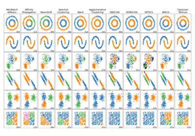
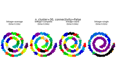
مقارنة خوارزميات التجميع المختلفة على مجموعات البيانات التجريبية