ملاحظة
Go to the end to download the full example code. or to run this example in your browser via JupyterLite or Binder
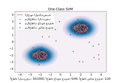
One-class SVM with non-linear kernel (RBF)#
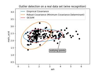
مثال لاستخدام SVM أحادي الفئة للكشف عن البيانات الشاذة.
One-class SVM هو خوارزمية غير مُشرفة تتعلم دالة اتخاذ القرار للكشف عن البيانات الشاذة: تصنيف البيانات الجديدة على أنها مشابهة أو مختلفة لمجموعة البيانات التدريبية.
# المؤلفون: مطوري مكتبة سكايلرن
# معرف الترخيص: BSD-3-Clause
import numpy as np
from sklearn import svm

# توليد بيانات التدريب
X = 0.3 * np.random.randn(100, 2)
X_train = np.r_[X + 2, X - 2]
# توليد بعض الملاحظات العادية الجديدة
X = 0.3 * np.random.randn(20, 2)
X_test = np.r_[X + 2, X - 2]
# توليد بعض الملاحظات الشاذة الجديدة
X_outliers = np.random.uniform(low=-4, high=4, size=(20, 2))

# تدريب النموذج
clf = svm.OneClassSVM(nu=0.1, kernel="rbf", gamma=0.1)
clf.fit(X_train)
y_pred_train = clf.predict(X_train)
y_pred_test = clf.predict(X_test)
y_pred_outliers = clf.predict(X_outliers)
n_error_train = y_pred_train[y_pred_train == -1].size
n_error_test = y_pred_test[y_pred_test == -1].size
n_error_outliers = y_pred_outliers[y_pred_outliers == 1].size
import matplotlib.font_manager
import matplotlib.lines as mlines
import matplotlib.pyplot as plt
from sklearn.inspection import DecisionBoundaryDisplay
_, ax = plt.subplots()
# توليد شبكة لعرض الحدود
xx, yy = np.meshgrid(np.linspace(-5, 5, 10), np.linspace(-5, 5, 10))
X = np.concatenate([xx.reshape(-1, 1), yy.reshape(-1, 1)], axis=1)
DecisionBoundaryDisplay.from_estimator(
clf,
X,
response_method="decision_function",
plot_method="contourf",
ax=ax,
cmap="PuBu",
)
DecisionBoundaryDisplay.from_estimator(
clf,
X,
response_method="decision_function",
plot_method="contourf",
ax=ax,
levels=[0, 10000],
colors="palevioletred",
)
DecisionBoundaryDisplay.from_estimator(
clf,
X,
response_method="decision_function",
plot_method="contour",
ax=ax,
levels=[0],
colors="darkred",
linewidths=2,
)
s = 40
b1 = ax.scatter(X_train[:, 0], X_train[:, 1], c="white", s=s, edgecolors="k")
b2 = ax.scatter(X_test[:, 0], X_test[:, 1], c="blueviolet", s=s, edgecolors="k")
c = ax.scatter(X_outliers[:, 0], X_outliers[:, 1], c="gold", s=s, edgecolors="k")
plt.legend(
[mlines.Line2D([], [], color="darkred"), b1, b2, c],
[
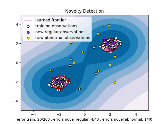
"learned frontier",
"training observations",
"new regular observations",
"new abnormal observations",
],
loc="upper left",
prop=matplotlib.font_manager.FontProperties(size=11),
)
ax.set(
xlabel=(
f"error train: {n_error_train}/200 ; errors novel regular: {n_error_test}/40 ;"
f" errors novel abnormal: {n_error_outliers}/40"
),
title="Novelty Detection",
xlim=(-5, 5),
ylim=(-5, 5),
)
plt.show()
Total running time of the script: (0 minutes 0.189 seconds)
Related examples
One-Class SVM مقابل One-Class SVM باستخدام Stochastic Gradient Descent
One-Class SVM مقابل One-Class SVM باستخدام Stochastic Gradient Descent
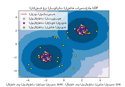
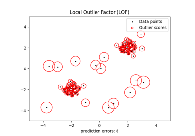
الكشف عن البيانات الشاذة باستخدام عامل الانحراف المحلي (LOF)
الكشف عن البيانات الشاذة باستخدام عامل الانحراف المحلي (LOF)
الكشف عن القيم الشاذة باستخدام عامل الانحراف المحلي (LOF)
الكشف عن القيم الشاذة باستخدام عامل الانحراف المحلي (LOF)