ملاحظة
Go to the end to download the full example code. or to run this example in your browser via JupyterLite or Binder
اختيار نموذج المزيج الغاوسي#
هذا المثال يوضح أنه يمكن إجراء اختيار النموذج باستخدام نماذج المزيج الغاوسي (GMM) باستخدام معايير نظرية المعلومات. يهتم اختيار النموذج بكل من نوع التغاير وعدد المكونات في النموذج.
في هذه الحالة، يوفر كل من معيار معلومات أكايكي (AIC) ومعيار معلومات بايز (BIC) النتيجة الصحيحة، ولكننا نقوم بعرض الأخير فقط لأن BIC أكثر ملاءمة لتحديد النموذج الحقيقي من بين مجموعة من المرشحين. على عكس الإجراءات البايزية، فإن هذه الاستدلالات خالية من المعايير المسبقة.
# المؤلفون: مطوري سكايلرن
# معرف الترخيص: BSD-3-Clause
توليد البيانات#
نقوم بتوليد مكونين (كل منهما يحتوي على n_samples) عن طريق أخذ عينات عشوائية
من التوزيع الطبيعي القياسي كما هو مُرجع من numpy.random.randn.
يتم الحفاظ على أحد المكونات كرويًا ولكن يتم تحويله وتغيير مقياسه. يتم تشويه المكون الآخر ليحصل على مصفوفة تغاير أكثر عمومية.
import numpy as np

n_samples = 500
np.random.seed(0)
C = np.array([[0.0, -0.1], [1.7, 0.4]])
component_1 = np.dot(np.random.randn(n_samples, 2), C)  # general
component_2 = 0.7 * np.random.randn(n_samples, 2) + np.array([-4, 1])  # spherical

X = np.concatenate([component_1, component_2])
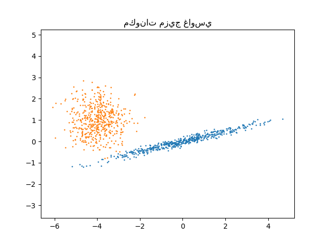
يمكننا تصور المكونات المختلفة:
import matplotlib.pyplot as plt

plt.scatter(component_1[:, 0], component_1[:, 1], s=0.8)
plt.scatter(component_2[:, 0], component_2[:, 1], s=0.8)
plt.title("مكونات مزيج غاوسي")
plt.axis("equal")
plt.show()
تدريب النموذج واختياره#
نقوم بتغيير عدد المكونات من 1 إلى 6 ونوع معاملات التغاير لاستخدامها:
"full": لكل مكون مصفوفة تغاير عامة خاصة به."tied": جميع المكونات تشترك في نفس مصفوفة التغاير العامة."diag": لكل مكون مصفوفة تغاير قطرية خاصة به."spherical": لكل مكون تغاير خاص به.
نقوم بتقييم النماذج المختلفة والاحتفاظ بأفضل نموذج (أقل BIC). يتم ذلك
باستخدام GridSearchCV ووظيفة تقييم
مُعرّفة من قبل المستخدم والتي تعيد نتيجة BIC السلبية، حيث أن
GridSearchCV مصممة ل**تحقيق الحد الأقصى**
لنتيجة التقييم (تحقيق الحد الأقصى للنتيجة السلبية لـ BIC يعادل تحقيق الحد
الأدنى لـ BIC).
يتم تخزين أفضل مجموعة من المعاملات والمقدر في best_parameters_ و
best_estimator_، على التوالي.
from sklearn.mixture import GaussianMixture
from sklearn.model_selection import GridSearchCV


def gmm_bic_score(estimator, X):
    """قابل للاستدعاء لتمريره إلى GridSearchCV والذي سيستخدم نتيجة BIC."""
    # اجعلها سلبية لأن GridSearchCV يتوقع نتيجة تقييم لتحقيق الحد الأقصى لها
    return -estimator.bic(X)


param_grid = {
    "n_components": range(1, 7),
    "covariance_type": ["spherical", "tied", "diag", "full"],
}
grid_search = GridSearchCV(
    GaussianMixture(), param_grid=param_grid, scoring=gmm_bic_score
)
grid_search.fit(X)
رسم نتائج BIC#
لتسهيل الرسم، يمكننا إنشاء pandas.DataFrame من نتائج
الاختبار المتقاطع الذي قام به البحث الشبكي. نقوم بإعادة عكس إشارة
نتيجة BIC لإظهار تأثير تحقيق الحد الأدنى منها.
import pandas as pd

df = pd.DataFrame(grid_search.cv_results_)[
    ["param_n_components", "param_covariance_type", "mean_test_score"]
]
df["mean_test_score"] = -df["mean_test_score"]
df = df.rename(
    columns={
        "param_n_components": "Number of components",
        "param_covariance_type": "Type of covariance",
        "mean_test_score": "BIC score",
    }
)
df.sort_values(by="BIC score").head()
import seaborn as sns

sns.catplot(
    data=df,
    kind="bar",
    x="Number of components",
    y="BIC score",
    hue="Type of covariance",
)
plt.show()
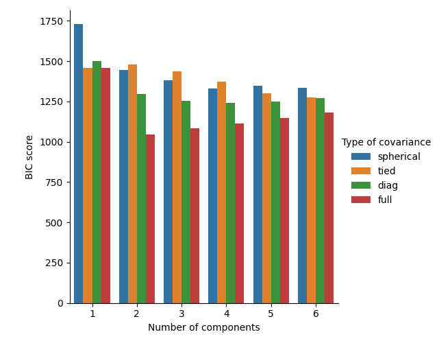
في الحالة الحالية، النموذج ذو المكونين وتغاير كامل (الذي يتوافق مع النموذج التوليدي الحقيقي) لديه أقل نتيجة BIC وبالتالي يتم اختياره من قبل البحث الشبكي.
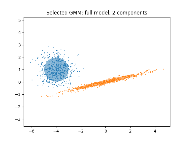
رسم أفضل نموذج#
نرsection
نرسم قطع ناقص لإظهار كل مكون غاوسي للنموذج المختار. لهذا الغرض،
نحتاج إلى إيجاد القيم الذاتية لمصفوفات التغاير كما هو مُرجع من الخاصية
covariances_. يعتمد شكل هذه المصفوفات على covariance_type:
"full": (n_components,n_features,n_features)"tied": (n_features,n_features)"diag": (n_components,n_features)"spherical": (n_components,)
from matplotlib.patches import Ellipse
from scipy import linalg

color_iter = sns.color_palette("tab10", 2)[::-1]
Y_ = grid_search.predict(X)

fig, ax = plt.subplots()

for i, (mean, cov, color) in enumerate(
    zip(
        grid_search.best_estimator_.means_,
        grid_search.best_estimator_.covariances_,
        color_iter,
    )
):
    v, w = linalg.eigh(cov)
    if not np.any(Y_ == i):
        continue
    plt.scatter(X[Y_ == i, 0], X[Y_ == i, 1], 0.8, color=color)

    angle = np.arctan2(w[0][1], w[0][0])
    angle = 180.0 * angle / np.pi  # تحويل إلى درجات
    v = 2.0 * np.sqrt(2.0) * np.sqrt(v)
    ellipse = Ellipse(mean, v[0], v[1], angle=180.0 + angle, color=color)
    ellipse.set_clip_box(fig.bbox)
    ellipse.set_alpha(0.5)
    ax.add_artist(ellipse)

plt.title(
    f"Selected GMM: {grid_search.best_params_['covariance_type']} model, "
    f"{grid_search.best_params_['n_components']} components"
)
plt.axis("equal")
plt.show()
Total running time of the script: (0 minutes 2.802 seconds)
Related examples
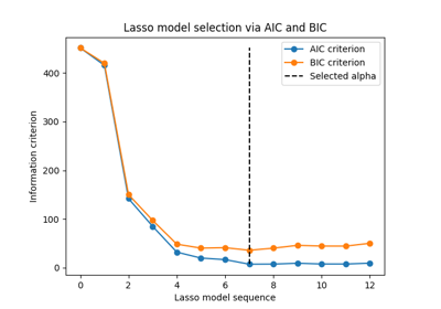
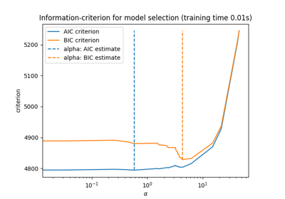
نموذج لاصو: اختيار النموذج باستخدام معايير AIC-BIC والتحقق المتقاطع