ملاحظة

Go to the end to download the full example code. or to run this example in your browser via JupyterLite or Binder

تقدير كثافة النواة البسيطة أحادية البعد#

يستخدم هذا المثال فئة KernelDensity لتوضيح مبادئ تقدير كثافة النواة في البعد أحادي.

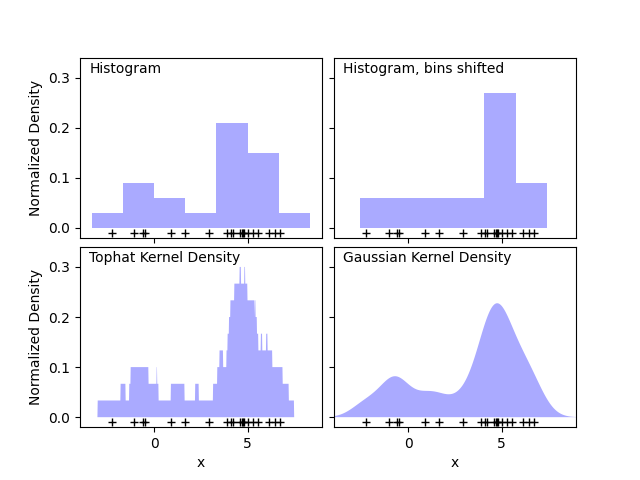
يوضح المخطط الأول أحد المشاكل المتعلقة باستخدام التوزيعات التكرارية لتصور كثافة النقاط في البعد أحادي. بديهياً، يمكن اعتبار التوزيع التكراري على أنه مخطط يتم فيه وضع "كتلة" وحدة فوق كل نقطة على شبكة منتظمة. ومع ذلك، كما توضح لوحتان العلويتان، يمكن أن يؤدي اختيار الشبكة لهذه الكتل إلى أفكار متباينة بشكل كبير حول الشكل الأساسي لتوزيع الكثافة. إذا قمنا بدلاً من ذلك بتركيز كل كتلة على النقطة التي تمثلها، فإننا نحصل على التقدير الموضح في اللوحة السفلية اليسرى. هذا هو تقدير كثافة النواة مع نواة "قبعة علوية". يمكن تعميم هذه الفكرة على أشكال نواة أخرى: توضح اللوحة السفلية اليمنى من الشكل الأول تقدير كثافة النواة الغاوسية على نفس التوزيع.

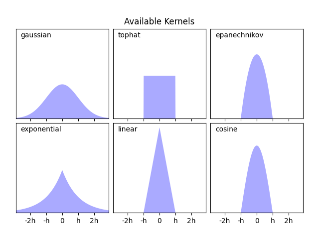
ينفذ Scikit-learn تقدير كثافة النواة بكفاءة باستخدام إما بنية شجرة الكرة أو شجرة KD، من خلال KernelDensity estimator. يتم عرض النواة المتاحة في الشكل الثاني من هذا المثال.

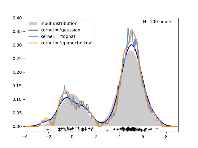
يقارن الشكل الثالث تقديرات كثافة النواة لتوزيع 100 عينة في البعد أحادي. على الرغم من أن هذا المثال يستخدم توزيعات أحادية البعد، إلا أن تقدير كثافة النواة يمكن تمديده بسهولة وكفاءة إلى أبعاد أعلى أيضًا.

# المؤلفون: مطوري scikit-learn
# معرف الترخيص: BSD-3-Clause

import matplotlib.pyplot as plt
import numpy as np
from scipy.stats import norm

from sklearn.neighbors import KernelDensity

# ----------------------------------------------------------------------
# رسم تطور التوزيعات التكرارية إلى نواة
np.random.seed(1)
N = 20
X = np.concatenate(
    (np.random.normal(0, 1, int(0.3 * N)), np.random.normal(5, 1, int(0.7 * N)))
)[:, np.newaxis]
X_plot = np.linspace(-5, 10, 1000)[:, np.newaxis]
bins = np.linspace(-5, 10, 10)

fig, ax = plt.subplots(2, 2, sharex=True, sharey=True)
fig.subplots_adjust(hspace=0.05, wspace=0.05)

# التوزيع التكراري 1
ax[0, 0].hist(X[:, 0], bins=bins, fc="#AAAAFF", density=True)
ax[0, 0].text(-3.5, 0.31, "Histogram")

# التوزيع التكراري 2
ax[0, 1].hist(X[:, 0], bins=bins + 0.75, fc="#AAAAFF", density=True)
ax[0, 1].text(-3.5, 0.31, "Histogram, bins shifted")

# تقدير كثافة النواة "قبعة علوية"
kde = KernelDensity(kernel="tophat", bandwidth=0.75).fit(X)
log_dens = kde.score_samples(X_plot)
ax[1, 0].fill(X_plot[:, 0], np.exp(log_dens), fc="#AAAAFF")
ax[1, 0].text(-3.5, 0.31, "Tophat Kernel Density")

# تقدير كثافة النواة الغاوسية
kde = KernelDensity(kernel="gaussian", bandwidth=0.75).fit(X)
log_dens = kde.score_samples(X_plot)
ax[1, 1].fill(X_plot[:, 0], np.exp(log_dens), fc="#AAAAFF")
ax[1, 1].text(-3.5, 0.31, "Gaussian Kernel Density")

for axi in ax.ravel():
    axi.plot(X[:, 0], np.full(X.shape[0], -0.01), "+k")
    axi.set_xlim(-4, 9)
    axi.set_ylim(-0.02, 0.34)

for axi in ax[:, 0]:
    axi.set_ylabel("Normalized Density")

for axi in ax[1, :]:
    axi.set_xlabel("x")

# ----------------------------------------------------------------------
# رسم جميع النواة المتاحة
X_plot = np.linspace(-6, 6, 1000)[:, None]
X_src = np.zeros((1, 1))

fig, ax = plt.subplots(2, 3, sharex=True, sharey=True)
fig.subplots_adjust(left=0.05, right=0.95, hspace=0.05, wspace=0.05)


def format_func(x, loc):
    if x == 0:
        return "0"
    elif x == 1:
        return "h"
    elif x == -1:
        return "-h"
    else:
        return "%ih" % x


for i, kernel in enumerate(
    ["gaussian", "tophat", "epanechnikov", "exponential", "linear", "cosine"]
):
    axi = ax.ravel()[i]
    log_dens = KernelDensity(kernel=kernel).fit(X_src).score_samples(X_plot)
    axi.fill(X_plot[:, 0], np.exp(log_dens), "-k", fc="#AAAAFF")
    axi.text(-2.6, 0.95, kernel)

    axi.xaxis.set_major_formatter(plt.FuncFormatter(format_func))
    axi.xaxis.set_major_locator(plt.MultipleLocator(1))
    axi.yaxis.set_major_locator(plt.NullLocator())

    axi.set_ylim(0, 1.05)
    axi.set_xlim(-2.9, 2.9)

ax[0, 1].set_title("Available Kernels")

# ----------------------------------------------------------------------
# رسم مثال على كثافة أحادية البعد
N = 100
np.random.seed(1)
X = np.concatenate(
    (np.random.normal(0, 1, int(0.3 * N)), np.random.normal(5, 1, int(0.7 * N)))
)[:, np.newaxis]

X_plot = np.linspace(-5, 10, 1000)[:, np.newaxis]

true_dens = 0.3 * norm(0, 1).pdf(X_plot[:, 0]) + 0.7 * norm(5, 1).pdf(X_plot[:, 0])

fig, ax = plt.subplots()
ax.fill(X_plot[:, 0], true_dens, fc="black", alpha=0.2, label="input distribution")
colors = ["navy", "cornflowerblue", "darkorange"]
kernels = ["gaussian", "tophat", "epanechnikov"]
lw = 2

for color, kernel in zip(colors, kernels):
    kde = KernelDensity(kernel=kernel, bandwidth=0.5).fit(X)
    log_dens = kde.score_samples(X_plot)
    ax.plot(
        X_plot[:, 0],
        np.exp(log_dens),
        color=color,
        lw=lw,
        linestyle="-",
        label="kernel = '{0}'".format(kernel),
    )

ax.text(6, 0.38, "N={0} points".format(N))

ax.legend(loc="upper left")
ax.plot(X[:, 0], -0.005 - 0.01 * np.random.random(X.shape[0]), "+k")

ax.set_xlim(-4, 9)
ax.set_ylim(-0.02, 0.4)
plt.show()