ملاحظة

Go to the end to download the full example code. or to run this example in your browser via JupyterLite or Binder

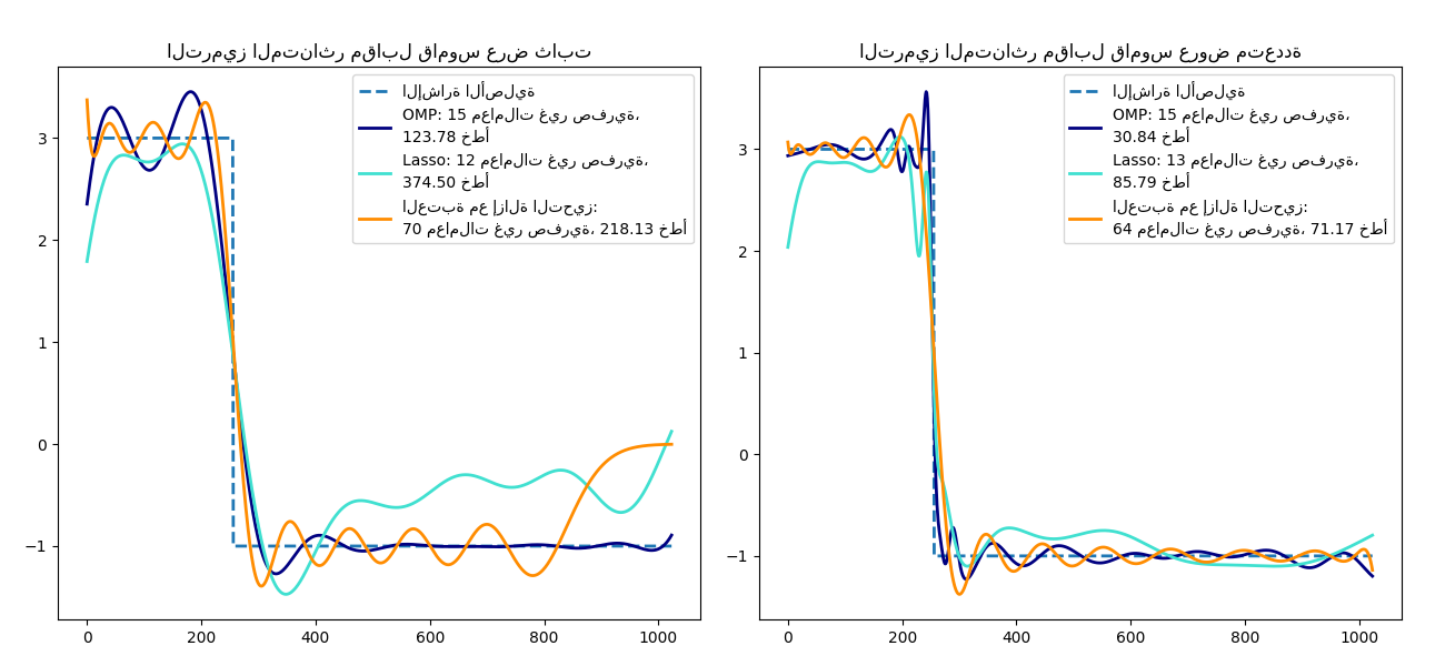
الترميز المتناثر مع قاموس محسوب مسبقًا#

تحويل إشارة كمزيج متناثر من مويجات Ricker. يقارن هذا المثال بصريًا طرق الترميز المتناثر المختلفة باستخدام مقدر SparseCoder. إن مويجة Ricker (المعروفة أيضًا باسم القبعة المكسيكية أو المشتقة الثانية لدالة غاوسية) ليست نواة جيدة بشكل خاص لتمثيل الإشارات الثابتة متعددة التعريف مثل هذه الإشارة. لذلك يمكن ملاحظة مدى أهمية إضافة عروض مختلفة من الذرات، وبالتالي يحفز ذلك على تعلم القاموس ليناسب نوع الإشارات الخاصة بك على أفضل وجه.

القاموس الأكثر ثراءً على اليمين ليس أكبر في الحجم، ويتم إجراء أخذ عينات فرعية أثقل من أجل البقاء في نفس ترتيب الحجم.

الترميز المتناثر مقابل قاموس عرض ثابت, الترميز المتناثر مقابل قاموس عروض متعددة

# Authors: The scikit-learn developers
# SPDX-License-Identifier: BSD-3-Clause

import matplotlib.pyplot as plt
import numpy as np

from sklearn.decomposition import SparseCoder


def ricker_function(resolution, center, width):
    """مويجة Ricker (القبعة المكسيكية) الفرعية المتقطعة"""
    x = np.linspace(0, resolution - 1, resolution)
    x = (
        (2 / (np.sqrt(3 * width) * np.pi**0.25))
        * (1 - (x - center) ** 2 / width**2)
        * np.exp(-((x - center) ** 2) / (2 * width**2))
    )
    return x


def ricker_matrix(width, resolution, n_components):
    """قاموس مويجات Ricker (القبعة المكسيكية)"""
    centers = np.linspace(0, resolution - 1, n_components)
    D = np.empty((n_components, resolution))
    for i, center in enumerate(centers):
        D[i] = ricker_function(resolution, center, width)
    D /= np.sqrt(np.sum(D**2, axis=1))[:, np.newaxis]
    return D


resolution = 1024
subsampling = 3  # معامل أخذ العينات الفرعية
width = 100
n_components = resolution // subsampling

# حساب قاموس المويجات
D_fixed = ricker_matrix(
    width=width, resolution=resolution, n_components=n_components)
D_multi = np.r_[
    tuple(
        ricker_matrix(width=w, resolution=resolution,
                      n_components=n_components // 5)
        for w in (10, 50, 100, 500, 1000)
    )
]

# إنشاء إشارة
y = np.linspace(0, resolution - 1, resolution)
first_quarter = y < resolution / 4
y[first_quarter] = 3.0
y[np.logical_not(first_quarter)] = -1.0

# سرد طرق الترميز المتناثر المختلفة بالتنسيق التالي:
# (العنوان، خوارزمية التحويل، ألفا التحويل،
#  معاملات التحويل غير الصفرية، اللون)
estimators = [
    ("OMP", "omp", None, 15, "navy"),
    ("Lasso", "lasso_lars", 2, None, "turquoise"),
]
lw = 2

plt.figure(figsize=(13, 6))
for subplot, (D, title) in enumerate(
    zip((D_fixed, D_multi), ("عرض ثابت", "عروض متعددة"))
):
    plt.subplot(1, 2, subplot + 1)
    plt.title("الترميز المتناثر مقابل قاموس %s" % title)
    plt.plot(y, lw=lw, linestyle="--", label="الإشارة الأصلية")
    # إجراء تقريب مويجي
    for title, algo, alpha, n_nonzero, color in estimators:
        coder = SparseCoder(
            dictionary=D,
            transform_n_nonzero_coefs=n_nonzero,
            transform_alpha=alpha,
            transform_algorithm=algo,
        )
        x = coder.transform(y.reshape(1, -1))
        density = len(np.flatnonzero(x))
        x = np.ravel(np.dot(x, D))
        squared_error = np.sum((y - x) ** 2)
        plt.plot(
            x,
            color=color,
            lw=lw,
            label="%s: %s معاملات غير صفرية،\n%.2f خطأ" % (
                title, density, squared_error),
        )

    # إزالة تحيز العتبة الناعمة
    coder = SparseCoder(
        dictionary=D, transform_algorithm="threshold", transform_alpha=20
    )
    x = coder.transform(y.reshape(1, -1))
    _, idx = np.where(x != 0)
    x[0, idx], _, _, _ = np.linalg.lstsq(D[idx, :].T, y, rcond=None)
    x = np.ravel(np.dot(x, D))
    squared_error = np.sum((y - x) ** 2)
    plt.plot(
        x,
        color="darkorange",
        lw=lw,
        label="العتبة مع إزالة التحيز:\n%d معاملات غير صفرية، %.2f خطأ"
        % (len(idx), squared_error),
    )
    plt.axis("tight")
    plt.legend(shadow=False, loc="best")
plt.subplots_adjust(0.04, 0.07, 0.97, 0.90, 0.09, 0.2)
plt.show()