ملاحظة

Go to the end to download the full example code. or to run this example in your browser via JupyterLite or Binder

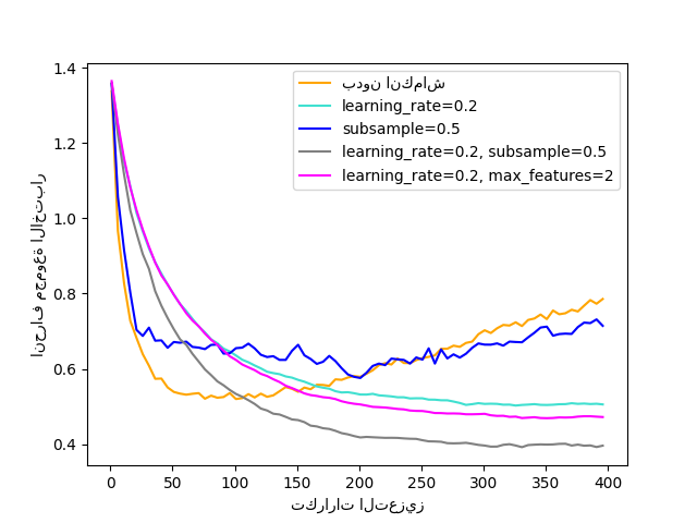
تنظيم التعزيز المتدرج#

توضيح لتأثير استراتيجيات تنظيم مختلفة للتعزيز المتدرج. المثال مأخوذ من Hastie et al 2009 [1].

دالة الخسارة المستخدمة هي انحراف ذو الحدين. التنظيم عبر الانكماش (learning_rate < 1.0) يحسن الأداء بشكل كبير. بالتزامن مع الانكماش، يمكن أن ينتج التعزيز المتدرج العشوائي (subsample < 1.0) نماذج أكثر دقة عن طريق تقليل التباين عبر التجميع. عادةً ما يؤدي الاختزال الفرعي بدون انكماش إلى أداء ضعيف. هناك إستراتيجية أخرى لتقليل التباين وهي عن طريق الاختزال الفرعي للميزات على غرار التقسيمات العشوائية في الغابات العشوائية (عبر معلمة max_features).

# Authors: The scikit-learn developers
# SPDX-License-Identifier: BSD-3-Clause

import matplotlib.pyplot as plt
import numpy as np

from sklearn import datasets, ensemble
from sklearn.metrics import log_loss
from sklearn.model_selection import train_test_split

X, y = datasets.make_hastie_10_2(n_samples=4000, random_state=1)

# تعيين التصنيفات من {-1, 1} إلى {0, 1}
labels, y = np.unique(y, return_inverse=True)

X_train, X_test, y_train, y_test = train_test_split(X, y, test_size=0.8, random_state=0)

original_params = {
    "n_estimators": 400,
    "max_leaf_nodes": 4,
    "max_depth": None,
    "random_state": 2,
    "min_samples_split": 5,
}

plt.figure()

for label, color, setting in [
    ("بدون انكماش", "orange", {"learning_rate": 1.0, "subsample": 1.0}),
    ("learning_rate=0.2", "turquoise", {"learning_rate": 0.2, "subsample": 1.0}),
    ("subsample=0.5", "blue", {"learning_rate": 1.0, "subsample": 0.5}),
    (
        "learning_rate=0.2, subsample=0.5",
        "gray",
        {"learning_rate": 0.2, "subsample": 0.5},
    ),
    (
        "learning_rate=0.2, max_features=2",
        "magenta",
        {"learning_rate": 0.2, "max_features": 2},
    ),
]:
    params = dict(original_params)
    params.update(setting)

    clf = ensemble.GradientBoostingClassifier(**params)
    clf.fit(X_train, y_train)

    # حساب انحراف مجموعة الاختبار
    test_deviance = np.zeros((params["n_estimators"],), dtype=np.float64)

    for i, y_proba in enumerate(clf.staged_predict_proba(X_test)):
        test_deviance[i] = 2 * log_loss(y_test, y_proba[:, 1])

    plt.plot(
        (np.arange(test_deviance.shape[0]) + 1)[::5],
        test_deviance[::5],
        "-",
        color=color,
        label=label,
    )

plt.legend(loc="upper right")
plt.xlabel("تكرارات التعزيز")
plt.ylabel("انحراف مجموعة الاختبار")

plt.show()