ملاحظة

Go to the end to download the full example code. or to run this example in your browser via JupyterLite or Binder

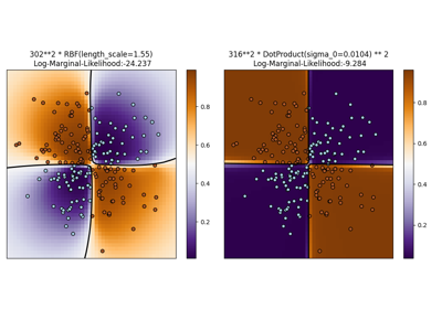
خطوط تساوي الاحتمال لتصنيف العمليات الغاوسية (GPC)#

مثال تصنيف ثنائي الأبعاد يوضح خطوط تساوي الاحتمال للاحتمالات المتوقعة.

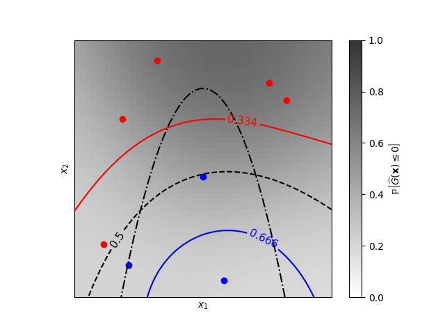
النواة المتعلمة: 0.0256**2 * DotProduct(sigma_0=5.72) ** 2

# Authors: The scikit-learn developers
# SPDX-License-Identifier: BSD-3-Clause

import numpy as np
from matplotlib import cm
from matplotlib import pyplot as plt

from sklearn.gaussian_process import GaussianProcessClassifier
from sklearn.gaussian_process.kernels import ConstantKernel as C
from sklearn.gaussian_process.kernels import DotProduct

# بعض الثوابت
lim = 8


def g(x):
    """الدالة المراد التنبؤ بها (سيتكون التصنيف بعد ذلك من التنبؤ
    بما إذا كانت g(x) <= 0 أم لا)"""
    return 5.0 - x[:, 1] - 0.5 * x[:, 0] ** 2.0


# تصميم التجارب
X = np.array(
    [
        [-4.61611719, -6.00099547],
        [4.10469096, 5.32782448],
        [0.00000000, -0.50000000],
        [-6.17289014, -4.6984743],
        [1.3109306, -6.93271427],
        [-5.03823144, 3.10584743],
        [-2.87600388, 6.74310541],
        [5.21301203, 4.26386883],
    ]
)

# الملاحظات
y = np.array(g(X) > 0, dtype=int)

# تهيئة وملاءمة نموذج العملية الغاوسية
kernel = C(0.1, (1e-5, np.inf)) * DotProduct(sigma_0=0.1) ** 2
gp = GaussianProcessClassifier(kernel=kernel)
gp.fit(X, y)
print("النواة المتعلمة: %s " % gp.kernel_)

# تقييم الدالة الحقيقية والاحتمال المتوقع
res = 50
x1, x2 = np.meshgrid(np.linspace(-lim, lim, res), np.linspace(-lim, lim, res))
xx = np.vstack([x1.reshape(x1.size), x2.reshape(x2.size)]).T

y_true = g(xx)
y_prob = gp.predict_proba(xx)[:, 1]
y_true = y_true.reshape((res, res))
y_prob = y_prob.reshape((res, res))

# رسم قيم التساوي الاحتمالية للتصنيف الاحتمالي
fig = plt.figure(1)
ax = fig.gca()
ax.axes.set_aspect("equal")
plt.xticks([])
plt.yticks([])
ax.set_xticklabels([])
ax.set_yticklabels([])
plt.xlabel("$x_1$")
plt.ylabel("$x_2$")

cax = plt.imshow(y_prob, cmap=cm.gray_r, alpha=0.8, extent=(-lim, lim, -lim, lim))
norm = plt.matplotlib.colors.Normalize(vmin=0.0, vmax=0.9)
cb = plt.colorbar(cax, ticks=[0.0, 0.2, 0.4, 0.6, 0.8, 1.0], norm=norm)
cb.set_label(r"${\rm \mathbb{P}}\left[\widehat{G}(\mathbf{x}) \leq 0\right]$")  # وصف شريط الألوان
plt.clim(0, 1)

plt.plot(X[y <= 0, 0], X[y <= 0, 1], "r.", markersize=12)

plt.plot(X[y > 0, 0], X[y > 0, 1], "b.", markersize=12)

plt.contour(x1, x2, y_true, [0.0], colors="k", linestyles="dashdot")

cs = plt.contour(x1, x2, y_prob, [0.666], colors="b", linestyles="solid")
plt.clabel(cs, fontsize=11)

cs = plt.contour(x1, x2, y_prob, [0.5], colors="k", linestyles="dashed")
plt.clabel(cs, fontsize=11)

cs = plt.contour(x1, x2, y_prob, [0.334], colors="r", linestyles="solid")
plt.clabel(cs, fontsize=11)

plt.show()