ملاحظة

Go to the end to download the full example code. or to run this example in your browser via JupyterLite or Binder

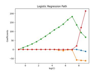
عقوبة L1 والندرة في الانحدار اللوجستي#

مقارنة الندرة (نسبة المعاملات الصفرية) للحلول عند استخدام عقوبة L1 و L2 و Elastic-Net لقيم مختلفة من C. يمكننا أن نرى أن القيم الكبيرة من C تعطي المزيد من الحرية للنموذج. على العكس من ذلك، القيم الأصغر من C تقيد النموذج أكثر. في حالة عقوبة L1، يؤدي ذلك إلى حلول أكثر ندرة. كما هو متوقع، ندرة عقوبة Elastic-Net تقع بين عقوبة L1 و L2.

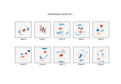
نصنف الصور 8x8 من الأرقام إلى فئتين: 0-4 مقابل 5-9. يوضح التصور معاملات النماذج لقيم C المختلفة.

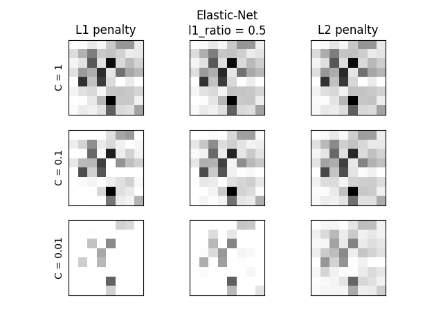
L1 penalty, Elastic-Net l1_ratio = 0.5, L2 penalty

C=1.00
Sparsity with L1 penalty:                6.25%
Sparsity with Elastic-Net penalty:       4.69%
Sparsity with L2 penalty:                4.69%
Score with L1 penalty:                   0.90
Score with Elastic-Net penalty:          0.90
Score with L2 penalty:                   0.90
C=0.10
Sparsity with L1 penalty:                29.69%
Sparsity with Elastic-Net penalty:       14.06%
Sparsity with L2 penalty:                4.69%
Score with L1 penalty:                   0.90
Score with Elastic-Net penalty:          0.90
Score with L2 penalty:                   0.90
C=0.01
Sparsity with L1 penalty:                84.38%
Sparsity with Elastic-Net penalty:       68.75%
Sparsity with L2 penalty:                4.69%
Score with L1 penalty:                   0.86
Score with Elastic-Net penalty:          0.88
Score with L2 penalty:                   0.89

# المؤلفون: مطوري سكايلرن
# معرف الترخيص: BSD-3-Clause

import matplotlib.pyplot as plt
import numpy as np

from sklearn import datasets
from sklearn.linear_model import LogisticRegression
from sklearn.preprocessing import StandardScaler

X, y = datasets.load_digits(return_X_y=True)

X = StandardScaler().fit_transform(X)

# تصنيف الأرقام الصغيرة مقابل الكبيرة
y = (y > 4).astype(int)

l1_ratio = 0.5  # وزن L1 في الانتظام Elastic-Net

fig, axes = plt.subplots(3, 3)

# تعيين معلمة الانتظام
for i, (C, axes_row) in enumerate(zip((1, 0.1, 0.01), axes)):
    # زيادة التحمل لوقت تدريب قصير
    clf_l1_LR = LogisticRegression(C=C, penalty="l1", tol=0.01, solver="saga")
    clf_l2_LR = LogisticRegression(C=C, penalty="l2", tol=0.01, solver="saga")
    clf_en_LR = LogisticRegression(
        C=C, penalty="elasticnet", solver="saga", l1_ratio=l1_ratio, tol=0.01
    )
    clf_l1_LR.fit(X, y)
    clf_l2_LR.fit(X, y)
    clf_en_LR.fit(X, y)

    coef_l1_LR = clf_l1_LR.coef_.ravel()
    coef_l2_LR = clf_l2_LR.coef_.ravel()
    coef_en_LR = clf_en_LR.coef_.ravel()

    # coef_l1_LR يحتوي على أصفار بسبب
    # معيار الندرة L1

    sparsity_l1_LR = np.mean(coef_l1_LR == 0) * 100
    sparsity_l2_LR = np.mean(coef_l2_LR == 0) * 100
    sparsity_en_LR = np.mean(coef_en_LR == 0) * 100

    print(f"C={C:.2f}")
    print(f"{'Sparsity with L1 penalty:':<40} {sparsity_l1_LR:.2f}%")
    print(f"{'Sparsity with Elastic-Net penalty:':<40} {sparsity_en_LR:.2f}%")
    print(f"{'Sparsity with L2 penalty:':<40} {sparsity_l2_LR:.2f}%")
    print(f"{'Score with L1 penalty:':<40} {clf_l1_LR.score(X, y):.2f}")
    print(f"{'Score with Elastic-Net penalty:':<40} {clf_en_LR.score(X, y):.2f}")
    print(f"{'Score with L2 penalty:':<40} {clf_l2_LR.score(X, y):.2f}")

    if i == 0:
        axes_row[0].set_title("L1 penalty")
        axes_row[1].set_title("Elastic-Net\nl1_ratio = %s" % l1_ratio)
        axes_row[2].set_title("L2 penalty")

    for ax, coefs in zip(axes_row, [coef_l1_LR, coef_en_LR, coef_l2_LR]):
        ax.imshow(
            np.abs(coefs.reshape(8, 8)),
            interpolation="nearest",
            cmap="binary",
            vmax=1,
            vmin=0,
        )
        ax.set_xticks(())
        ax.set_yticks(())

    axes_row[0].set_ylabel(f"C = {C}")

plt.show()