ملاحظة

Go to the end to download the full example code. or to run this example in your browser via JupyterLite or Binder

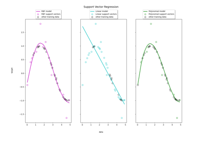
مقارنة بين الانحدار النووي المنتظم والانحدار الداعم للمتجهات#

كل من الانحدار النووي المنتظم (KRR) والانحدار الداعم للمتجهات (SVR) يتعلمان دالة غير خطية من خلال استخدام خدعة النواة، أي أنهما يتعلمان دالة خطية في الفضاء الذي تسببه النواة المقابلة، والتي تقابل دالة غير خطية في المساحة الأصلية. يختلفان في دالات الخسارة (ridge مقابل epsilon-insensitive loss). على عكس الانحدار الداعم للمتجهات، يمكن إجراء الانحدار النووي المنتظم في شكل مغلق وعادة ما يكون أسرع للمجموعات المتوسطة الحجم. من ناحية أخرى، فإن النموذج المُتعلم غير متفرق، وبالتالي فهو أبطأ من الانحدار الداعم للمتجهات في وقت التنبؤ.

يوضح هذا المثال كلتا الطريقتين على مجموعة بيانات اصطناعية، والتي تتكون من دالة هدف جيبية وضوضاء قوية تضاف إلى كل نقطة بيانات خامسة.

المؤلفون: مطوري سكايلرن معرف الترخيص: BSD-3-Clause

توليد بيانات العينة#

import numpy as np
rng = np.random.RandomState(42)

X = 5 * rng.rand(10000, 1)
y = np.sin(X).ravel()

# أضف ضوضاء إلى الأهداف
y[::5] += 3 * (0.5 - rng.rand(X.shape[0] // 5))

X_plot = np.linspace(0, 5, 100000)[:, None]

إنشاء نماذج الانحدار القائمة على النواة#

from sklearn.kernel_ridge import KernelRidge
from sklearn.model_selection import GridSearchCV
from sklearn.svm import SVR

train_size = 100

svr = GridSearchCV(
    SVR(kernel="rbf", gamma=0.1),
    param_grid={"C": [1e0, 1e1, 1e2, 1e3], "gamma": np.logspace(-2, 2, 5)},
)

kr = GridSearchCV(
    KernelRidge(kernel="rbf", gamma=0.1),
    param_grid={"alpha": [1e0, 0.1, 1e-2, 1e-3], "gamma": np.logspace(-2, 2, 5)},
)

مقارنة أوقات الانحدار الداعم للمتجهات والانحدار النووي المنتظم#

import time

t0 = time.time()
svr.fit(X[:train_size], y[:train_size])
svr_fit = time.time() - t0
print(f"Best SVR with params: {svr.best_params_} and R2 score: {svr.best_score_:.3f}")
print("SVR complexity and bandwidth selected and model fitted in %.3f s" % svr_fit)

t0 = time.time()
kr.fit(X[:train_size], y[:train_size])
kr_fit = time.time() - t0
print(f"Best KRR with params: {kr.best_params_} and R2 score: {kr.best_score_:.3f}")
print("KRR complexity and bandwidth selected and model fitted in %.3f s" % kr_fit)

sv_ratio = svr.best_estimator_.support_.shape[0] / train_size
print("Support vector ratio: %.3f" % sv_ratio)

t0 = time.time()
y_svr = svr.predict(X_plot)
svr_predict = time.time() - t0
print("SVR prediction for %d inputs in %.3f s" % (X_plot.shape[0], svr_predict))

t0 = time.time()
y_kr = kr.predict(X_plot)
kr_predict = time.time() - t0
print("KRR prediction for %d inputs in %.3f s" % (X_plot.shape[0], kr_predict))

Best SVR with params: {'C': 1.0, 'gamma': np.float64(0.1)} and R2 score: 0.737
SVR complexity and bandwidth selected and model fitted in 0.592 s
Best KRR with params: {'alpha': 0.1, 'gamma': np.float64(0.1)} and R2 score: 0.723
KRR complexity and bandwidth selected and model fitted in 0.281 s
Support vector ratio: 0.340
SVR prediction for 100000 inputs in 0.118 s
KRR prediction for 100000 inputs in 0.121 s

النظر في النتائج#

import matplotlib.pyplot as plt

sv_ind = svr.best_estimator_.support_
plt.scatter(
    X[sv_ind],
    y[sv_ind],
    c="r",
    s=50,
    label="SVR support vectors",
    zorder=2,
    edgecolors=(0, 0, 0),
)
plt.scatter(X[:100], y[:100], c="k", label="data", zorder=1, edgecolors=(0, 0, 0))
plt.plot(
    X_plot,
    y_svr,
    c="r",
    label="SVR (fit: %.3fs, predict: %.3fs)" % (svr_fit, svr_predict),
)
plt.plot(
    X_plot, y_kr, c="g", label="KRR (fit: %.3fs, predict: %.3fs)" % (kr_fit, kr_predict)
)
plt.xlabel("data")
plt.ylabel("target")
plt.title("SVR versus Kernel Ridge")
_ = plt.legend()

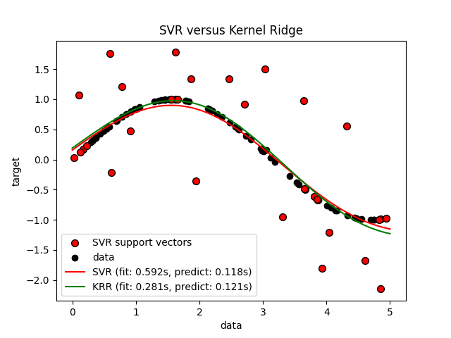
الشكل السابق يقارن النموذج المُتعلم للانحدار النووي المنتظم والانحدار الداعم للمتجهات عندما يكون كل من التعقيد/الانتظام وعرض نطاق نواة RBF مُحسن باستخدام grid-search. الدالات المُتعلمة متشابهة جداً؛ ومع ذلك، فإن الانحدار النووي المنتظم أسرع تقريباً 3-4 مرات من الانحدار الداعم للمتجهات (كلاهما مع grid-search).

يمكن أن يكون التنبؤ بـ 100000 قيمة مستهدفة في النظرية تقريباً ثلاثة مرات أسرع مع الانحدار الداعم للمتجهات منذ أنه تعلم نموذج متفرق باستخدام فقط تقريباً 1/3 من نقاط البيانات التدريبية كمتجهات دعم. ومع ذلك، في الممارسة، هذا ليس بالضرورة هو الحال بسبب تفاصيل التنفيذ في الطريقة التي يتم بها حساب دالة النواة لكل نموذج والتي يمكن أن تجعل نموذج الانحدار النووي المنتظم سريعًا أو حتى أسرع على الرغم من إجراء المزيد من العمليات الحسابية.

تصور أوقات التدريب والتنبؤ#

plt.figure()

sizes = np.logspace(1, 3.8, 7).astype(int)
for name, estimator in {
    "KRR": KernelRidge(kernel="rbf", alpha=0.01, gamma=10),
    "SVR": SVR(kernel="rbf", C=1e2, gamma=10),
}.items():
    train_time = []
    test_time = []
    for train_test_size in sizes:
        t0 = time.time()
        estimator.fit(X[:train_test_size], y[:train_test_size])
        train_time.append(time.time() - t0)

        t0 = time.time()
        estimator.predict(X_plot[:1000])
        test_time.append(time.time() - t0)

    plt.plot(
        sizes,
        train_time,
        "o-",
        color="r" if name == "SVR" else "g",
        label="%s (train)" % name,
    )
    plt.plot(
        sizes,
        test_time,
        "o--",
        color="r" if name == "SVR" else "g",
        label="%s (test)" % name,
    )

plt.xscale("log")
plt.yscale("log")
plt.xlabel("Train size")
plt.ylabel("Time (seconds)")
plt.title("Execution Time")
_ = plt.legend(loc="best")

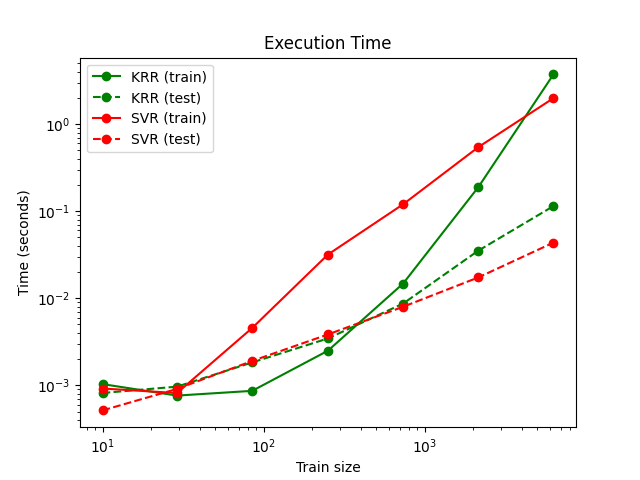
هذا الشكل يقارن الوقت اللازم للتدريب والتنبؤ للانحدار النووي المنتظم والانحدار الداعم للمتجهات لمختلف أحجام مجموعة التدريب. الانحدار النووي المنتظم أسرع من الانحدار الداعم للمتجهات لمجموعات التدريب المتوسطة الحجم (أقل من بضعة آلاف من العينات)؛ ومع ذلك، لمجموعات التدريب الأكبر، فإن الانحدار الداعم للمتجهات يتدرج بشكل أفضل. فيما يتعلق بوقت التنبؤ، يجب أن يكون الانحدار الداعم للمتجهات أسرع من الانحدار النووي المنتظم لجميع أحجام مجموعة التدريب بسبب الحل المتفرق المُتعلم، ومع ذلك، هذا ليس بالضرورة هو الحال في الممارسة بسبب تفاصيل التنفيذ. لاحظ أن درجة التفرق وبالتالي يعتمد وقت التنبؤ على معاملات الانحدار الداعم للمتجهات epsilon و C.

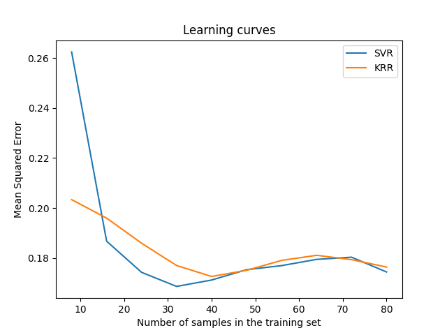
تصور منحنيات التعلم#

from sklearn.model_selection import LearningCurveDisplay

_, ax = plt.subplots()

svr = SVR(kernel="rbf", C=1e1, gamma=0.1)
kr = KernelRidge(kernel="rbf", alpha=0.1, gamma=0.1)

common_params = {
    "X": X[:100],
    "y": y[:100],
    "train_sizes": np.linspace(0.1, 1, 10),
    "scoring": "neg_mean_squared_error",
    "negate_score": True,
    "score_name": "Mean Squared Error",
    "score_type": "test",
    "std_display_style": None,
    "ax": ax,
}

LearningCurveDisplay.from_estimator(svr, **common_params)
LearningCurveDisplay.from_estimator(kr, **common_params)
ax.set_title("Learning curves")
ax.legend(handles=ax.get_legend_handles_labels()[0], labels=["SVR", "KRR"])

plt.show()