ملاحظة
Go to the end to download the full example code. or to run this example in your browser via JupyterLite or Binder
العنقدة الهرمية: العنقدة المنظمة وغير المنظمة#
مثال يبني مجموعة بيانات Swiss Roll ويقوم بتشغيل العنقدة الهرمية على موقعها.
لمزيد من المعلومات، راجع التجميع الهرمي.
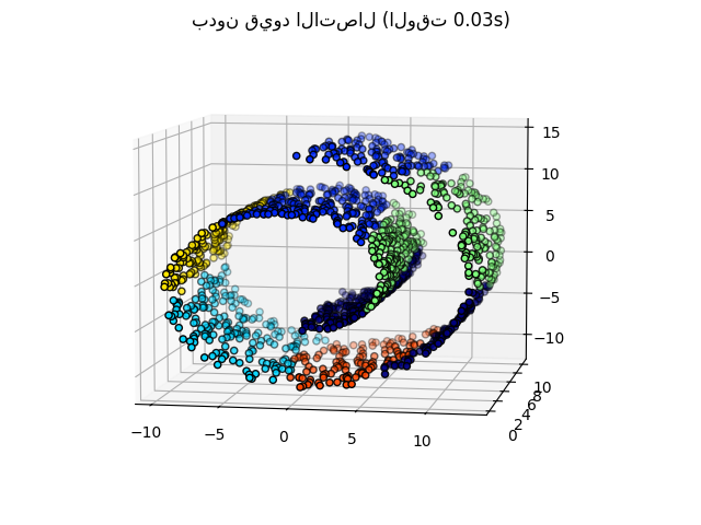
في الخطوة الأولى، يتم تنفيذ العنقدة الهرمية بدون قيود الاتصال على البنية وتستند فقط على المسافة، في حين أن في الخطوة الثانية، يتم تقييد العنقدة إلى رسم k-Nearest Neighbors البياني: إنها عنقدة هرمية ذات بنية مسبقة.
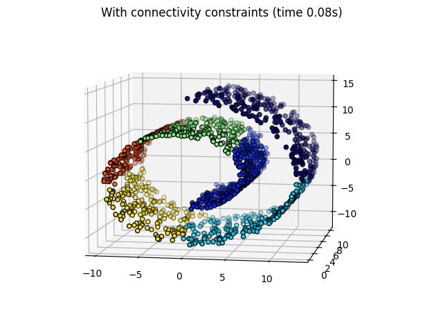
بعض المجموعات التي تم تعلمها بدون قيود الاتصال لا تحترم بنية Swiss Roll وتمتد عبر طيات مختلفة من الدوال. على العكس، عند معارضة قيود الاتصال، تشكل المجموعات تقسيمًا جيدًا لسويس رول.
# المؤلفون: مطوري scikit-learn
# معرف الترخيص: BSD-3-Clause

from sklearn.neighbors import kneighbors_graph
import matplotlib.pyplot as plt
from sklearn.cluster import AgglomerativeClustering
import time as time

# الاستيراد التالي مطلوب
# لعمل الإسقاط ثلاثي الأبعاد مع matplotlib < 3.2
import mpl_toolkits.mplot3d  # noqa: F401
import numpy as np
توليد البيانات#
نبدأ بتوليد مجموعة بيانات Swiss Roll.
from sklearn.datasets import make_swiss_roll

n_samples = 1500
noise = 0.05
X, _ = make_swiss_roll(n_samples, noise=noise)
# Make it thinner
X[:, 1] *= 0.5
حساب العنقدة#
نحن نؤدي AgglomerativeClustering الذي يأتي تحت العنقدة الهرمية بدون أي قيود اتصال.
print("Compute unstructured hierarchical clustering...")
st = time.time()
ward = AgglomerativeClustering(n_clusters=6, linkage="ward").fit(X)
elapsed_time = time.time() - st
label = ward.labels_
print(f"Elapsed time: {elapsed_time:.2f}s")
print(f"Number of points: {label.size}")
Compute unstructured hierarchical clustering...
Elapsed time: 0.03s
Number of points: 1500
رسم النتيجة#
رسم العنقدة الهرمية غير المنظمة.
fig1 = plt.figure()
ax1 = fig1.add_subplot(111, projection="3d", elev=7, azim=-80)
ax1.set_position([0, 0, 0.95, 1])
for l in np.unique(label):
    ax1.scatter(
        X[label == l, 0],
        X[label == l, 1],
        X[label == l, 2],
        color=plt.cm.jet(float(l) / np.max(label + 1)),
        s=20,
        edgecolor="k",
    )
_ = fig1.suptitle(f"بدون قيود الاتصال (الوقت {elapsed_time:.2f}s)")
نحن نحدد k-Nearest Neighbors مع 10 جيران#
connectivity = kneighbors_graph(X, n_neighbors=10, include_self=False)
حساب العنقدة#
نحن نؤدي AgglomerativeClustering مرة أخرى مع قيود الاتصال.
print("Compute structured hierarchical clustering...")
st = time.time()
ward = AgglomerativeClustering(
    n_clusters=6, connectivity=connectivity, linkage="ward"
).fit(X)
elapsed_time = time.time() - st
label = ward.labels_
print(f"Elapsed time: {elapsed_time:.2f}s")
print(f"Number of points: {label.size}")
Compute structured hierarchical clustering...
Elapsed time: 0.08s
Number of points: 1500
رسم النتيجة#
رسم العنقدة الهرمية المنظمة.
fig2 = plt.figure()
ax2 = fig2.add_subplot(121, projection="3d", elev=7, azim=-80)
ax2.set_position([0, 0, 0.95, 1])
for l in np.unique(label):
    ax2.scatter(
        X[label == l, 0],
        X[label == l, 1],
        X[label == l, 2],
        color=plt.cm.jet(float(l) / np.max(label + 1)),
        s=20,
        edgecolor="k",
    )
fig2.suptitle(f"With connectivity constraints (time {elapsed_time:.2f}s)")

plt.show()
Total running time of the script: (0 minutes 0.400 seconds)
Related examples
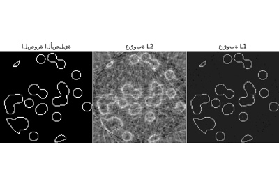
sphx_glr_auto_examples_applications_plot_tomography_l1_reconstruction.py
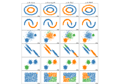
مقارنة طرق الربط الهرمي المختلفة على مجموعات بيانات تجريبية