ملاحظة

Go to the end to download the full example code. or to run this example in your browser via JupyterLite or Binder

Model-based and sequential feature selection#

يوضح هذا المثال ويقارن نهجين لاختيار الميزات: SelectFromModel الذي يعتمد على أهمية الميزات، و SequentialFeatureSelector الذي يعتمد على نهج جشع.

نستخدم مجموعة بيانات السكري، والتي تتكون من 10 ميزات تم جمعها من 442 مريضًا بالسكري.

Authors: Manoj Kumar, Maria Telenczuk, Nicolas Hug.

License: BSD 3 clause

# Authors: The scikit-learn developers
# SPDX-License-Identifier: BSD-3-Clause

تحميل البيانات#

نقوم أولاً بتحميل مجموعة بيانات السكري المتاحة من داخل scikit-learn، ونطبع وصفها:

from sklearn.datasets import load_diabetes

diabetes = load_diabetes()
X, y = diabetes.data, diabetes.target
print(diabetes.DESCR)

.. _diabetes_dataset:

Diabetes dataset
----------------

Ten baseline variables, age, sex, body mass index, average blood
pressure, and six blood serum measurements were obtained for each of n =
442 diabetes patients, as well as the response of interest, a
quantitative measure of disease progression one year after baseline.

**Data Set Characteristics:**

:Number of Instances: 442

:Number of Attributes: First 10 columns are numeric predictive values

:Target: Column 11 is a quantitative measure of disease progression one year after baseline

:Attribute Information:
    - age     age in years
    - sex
    - bmi     body mass index
    - bp      average blood pressure
    - s1      tc, total serum cholesterol
    - s2      ldl, low-density lipoproteins
    - s3      hdl, high-density lipoproteins
    - s4      tch, total cholesterol / HDL
    - s5      ltg, possibly log of serum triglycerides level
    - s6      glu, blood sugar level

Note: Each of these 10 feature variables have been mean centered and scaled by the standard deviation times the square root of `n_samples` (i.e. the sum of squares of each column totals 1).

Source URL:
https://www4.stat.ncsu.edu/~boos/var.select/diabetes.html

For more information see:
Bradley Efron, Trevor Hastie, Iain Johnstone and Robert Tibshirani (2004) "Least Angle Regression," Annals of Statistics (with discussion), 407-499.
(https://web.stanford.edu/~hastie/Papers/LARS/LeastAngle_2002.pdf)

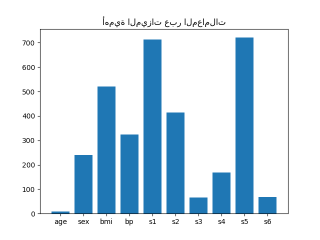
أهمية الميزات من المعاملات#

للحصول على فكرة عن أهمية الميزات، سنستخدم مقدّر RidgeCV. تعتبر الميزات ذات أعلى قيمة مطلقة لـ coef_ هي الأكثر أهمية. يمكننا ملاحظة المعاملات مباشرة دون الحاجة إلى تغيير مقياسها (أو تغيير مقياس البيانات) لأنه من الوصف أعلاه، نعلم أن الميزات قد تم توحيدها بالفعل. للحصول على مثال أكثر اكتمالاً عن تفسيرات معاملات النماذج الخطية، يمكنك الرجوع إلى المزالق الشائعة في تفسير معاملات النماذج الخطية. # noqa: E501

import matplotlib.pyplot as plt
import numpy as np

from sklearn.linear_model import RidgeCV

ridge = RidgeCV(alphas=np.logspace(-6, 6, num=5)).fit(X, y)
importance = np.abs(ridge.coef_)
feature_names = np.array(diabetes.feature_names)
plt.bar(height=importance, x=feature_names)
plt.title("أهمية الميزات عبر المعاملات")
plt.show()

تحديد الميزات بناءً على الأهمية#

الآن نريد تحديد الميزتين الأكثر أهمية وفقًا للمعاملات. SelectFromModel مخصصة لذلك فقط. SelectFromModel تقبل معلمة threshold وستحدد الميزات التي تكون أهميتها (المحددة بواسطة المعاملات) أعلى من هذه العتبة.

نظرًا لأننا نريد تحديد ميزتين فقط، فسنقوم بتعيين هذه العتبة أعلى بقليل من معامل ثالث أهم ميزة.

from time import time

from sklearn.feature_selection import SelectFromModel

threshold = np.sort(importance)[-3] + 0.01

tic = time()
sfm = SelectFromModel(ridge, threshold=threshold).fit(X, y)
toc = time()
print(f"الميزات المحددة بواسطة SelectFromModel: {feature_names[sfm.get_support()]}")
print(f"تم في {toc - tic:.3f}s")

الميزات المحددة بواسطة SelectFromModel: ['s1' 's5']
تم في 0.002s

تحديد الميزات مع اختيار الميزات المتسلسل#

هناك طريقة أخرى لتحديد الميزات وهي استخدام SequentialFeatureSelector (SFS). SFS هو إجراء جشع حيث، في كل تكرار، نختار أفضل ميزة جديدة لإضافتها إلى ميزاتنا المحددة بناءً على درجة التحقق المتبادل. أي أننا نبدأ بصفر ميزات ونختار أفضل ميزة واحدة بأعلى درجة. يتم تكرار الإجراء حتى نصل إلى العدد المطلوب من الميزات المحددة.

يمكننا أيضًا الانتقال في الاتجاه المعاكس (SFS للخلف)، أي البدء بجميع الميزات واختيار الميزات بشكل جشع لإزالتها واحدة تلو الأخرى. نوضح كلا النهجين هنا.

from sklearn.feature_selection import SequentialFeatureSelector

tic_fwd = time()
sfs_forward = SequentialFeatureSelector(
    ridge, n_features_to_select=2, direction="forward"
).fit(X, y)
toc_fwd = time()

tic_bwd = time()
sfs_backward = SequentialFeatureSelector(
    ridge, n_features_to_select=2, direction="backward"
).fit(X, y)
toc_bwd = time()

print(
    "الميزات المحددة بواسطة الاختيار المتسلسل للأمام: "
    f"{feature_names[sfs_forward.get_support()]}"
)
print(f"تم في {toc_fwd - tic_fwd:.3f}s")
print(
    "الميزات المحددة بواسطة الاختيار المتسلسل للخلف: "
    f"{feature_names[sfs_backward.get_support()]}"
)
print(f"تم في {toc_bwd - tic_bwd:.3f}s")

الميزات المحددة بواسطة الاختيار المتسلسل للأمام: ['bmi' 's5']
تم في 0.252s
الميزات المحددة بواسطة الاختيار المتسلسل للخلف: ['bmi' 's5']
تم في 0.720s

من المثير للاهتمام أن الاختيار الأمامي والخلفي قد حددا نفس مجموعة الميزات. بشكل عام، ليس هذا هو الحال وستؤدي الطريقتان إلى نتائج مختلفة.

نلاحظ أيضًا أن الميزات التي حددها SFS تختلف عن تلك التي حددتها أهمية الميزات: يحدد SFS bmi بدلاً من s1. يبدو هذا منطقيًا، نظرًا لأن bmi تتوافق مع ثالث أهم ميزة وفقًا للمعاملات. إنه أمر رائع للغاية بالنظر إلى أن SFS لا يستخدم المعاملات على الإطلاق.

في الختام، تجدر الإشارة إلى أن SelectFromModel أسرع بكثير من SFS. في الواقع، SelectFromModel تحتاج فقط إلى ملاءمة نموذج مرة واحدة، بينما يحتاج SFS إلى التحقق المتبادل للعديد من النماذج المختلفة لكل تكرار. ومع ذلك، يعمل SFS مع أي نموذج، بينما تتطلب SelectFromModel أن يعرض المقدّر الأساسي سمة coef_ أو سمة feature_importances_. يكون SFS الأمامي أسرع من SFS الخلفي لأنه يحتاج فقط إلى إجراء n_features_to_select = 2 تكرار، بينما يحتاج SFS الخلفي إلى إجراء n_features - n_features_to_select = 8 تكرار.

استخدام قيم التسامح السلبية#

SequentialFeatureSelector يمكن استخدامها لإزالة الميزات الموجودة في مجموعة البيانات وإرجاع مجموعة فرعية أصغر من الميزات الأصلية مع direction="backward" وقيمة سالبة لـ tol.

نبدأ بتحميل مجموعة بيانات سرطان الثدي، والتي تتكون من 30 ميزة مختلفة و 569 عينة.

import numpy as np

from sklearn.datasets import load_breast_cancer

breast_cancer_data = load_breast_cancer()
X, y = breast_cancer_data.data, breast_cancer_data.target
feature_names = np.array(breast_cancer_data.feature_names)
print(breast_cancer_data.DESCR)

.. _breast_cancer_dataset:

Breast cancer wisconsin (diagnostic) dataset
--------------------------------------------

**Data Set Characteristics:**

:Number of Instances: 569

:Number of Attributes: 30 numeric, predictive attributes and the class

:Attribute Information:
    - radius (mean of distances from center to points on the perimeter)
    - texture (standard deviation of gray-scale values)
    - perimeter
    - area
    - smoothness (local variation in radius lengths)
    - compactness (perimeter^2 / area - 1.0)
    - concavity (severity of concave portions of the contour)
    - concave points (number of concave portions of the contour)
    - symmetry
    - fractal dimension ("coastline approximation" - 1)

    The mean, standard error, and "worst" or largest (mean of the three
    worst/largest values) of these features were computed for each image,
    resulting in 30 features.  For instance, field 0 is Mean Radius, field
    10 is Radius SE, field 20 is Worst Radius.

    - class:
            - WDBC-Malignant
            - WDBC-Benign

:Summary Statistics:

===================================== ====== ======
                                        Min    Max
===================================== ====== ======
radius (mean):                        6.981  28.11
texture (mean):                       9.71   39.28
perimeter (mean):                     43.79  188.5
area (mean):                          143.5  2501.0
smoothness (mean):                    0.053  0.163
compactness (mean):                   0.019  0.345
concavity (mean):                     0.0    0.427
concave points (mean):                0.0    0.201
symmetry (mean):                      0.106  0.304
fractal dimension (mean):             0.05   0.097
radius (standard error):              0.112  2.873
texture (standard error):             0.36   4.885
perimeter (standard error):           0.757  21.98
area (standard error):                6.802  542.2
smoothness (standard error):          0.002  0.031
compactness (standard error):         0.002  0.135
concavity (standard error):           0.0    0.396
concave points (standard error):      0.0    0.053
symmetry (standard error):            0.008  0.079
fractal dimension (standard error):   0.001  0.03
radius (worst):                       7.93   36.04
texture (worst):                      12.02  49.54
perimeter (worst):                    50.41  251.2
area (worst):                         185.2  4254.0
smoothness (worst):                   0.071  0.223
compactness (worst):                  0.027  1.058
concavity (worst):                    0.0    1.252
concave points (worst):               0.0    0.291
symmetry (worst):                     0.156  0.664
fractal dimension (worst):            0.055  0.208
===================================== ====== ======

:Missing Attribute Values: None

:Class Distribution: 212 - Malignant, 357 - Benign

:Creator:  Dr. William H. Wolberg, W. Nick Street, Olvi L. Mangasarian

:Donor: Nick Street

:Date: November, 1995

This is a copy of UCI ML Breast Cancer Wisconsin (Diagnostic) datasets.
https://goo.gl/U2Uwz2

Features are computed from a digitized image of a fine needle
aspirate (FNA) of a breast mass.  They describe
characteristics of the cell nuclei present in the image.

Separating plane described above was obtained using
Multisurface Method-Tree (MSM-T) [K. P. Bennett, "Decision Tree
Construction Via Linear Programming." Proceedings of the 4th
Midwest Artificial Intelligence and Cognitive Science Society,
pp. 97-101, 1992], a classification method which uses linear
programming to construct a decision tree.  Relevant features
were selected using an exhaustive search in the space of 1-4
features and 1-3 separating planes.

The actual linear program used to obtain the separating plane
in the 3-dimensional space is that described in:
[K. P. Bennett and O. L. Mangasarian: "Robust Linear
Programming Discrimination of Two Linearly Inseparable Sets",
Optimization Methods and Software 1, 1992, 23-34].

This database is also available through the UW CS ftp server:

ftp ftp.cs.wisc.edu
cd math-prog/cpo-dataset/machine-learn/WDBC/

.. dropdown:: References

  - W.N. Street, W.H. Wolberg and O.L. Mangasarian. Nuclear feature extraction
    for breast tumor diagnosis. IS&T/SPIE 1993 International Symposium on
    Electronic Imaging: Science and Technology, volume 1905, pages 861-870,
    San Jose, CA, 1993.
  - O.L. Mangasarian, W.N. Street and W.H. Wolberg. Breast cancer diagnosis and
    prognosis via linear programming. Operations Research, 43(4), pages 570-577,
    July-August 1995.
  - W.H. Wolberg, W.N. Street, and O.L. Mangasarian. Machine learning techniques
    to diagnose breast cancer from fine-needle aspirates. Cancer Letters 77 (1994)
    163-171.

سنستخدم مقدّر LogisticRegression مع SequentialFeatureSelector لإجراء اختيار الميزات.

from sklearn.linear_model import LogisticRegression
from sklearn.metrics import roc_auc_score
from sklearn.pipeline import make_pipeline
from sklearn.preprocessing import StandardScaler

for tol in [-1e-2, -1e-3, -1e-4]:
    start = time()
    feature_selector = SequentialFeatureSelector(
        LogisticRegression(),
        n_features_to_select="auto",
        direction="backward",
        scoring="roc_auc",
        tol=tol,
        n_jobs=2,
    )
    model = make_pipeline(StandardScaler(), feature_selector, LogisticRegression())
    model.fit(X, y)
    end = time()
    print(f"\ntol: {tol}")
    print(f"الميزات المحددة: {feature_names[model[1].get_support()]}")
    print(f"درجة ROC AUC: {roc_auc_score(y, model.predict_proba(X)[:, 1]):.3f}")
    print(f"تم في {end - start:.3f}s")

tol: -0.01
الميزات المحددة: ['worst perimeter']
درجة ROC AUC: 0.975
تم في 14.650s

tol: -0.001
الميزات المحددة: ['radius error' 'fractal dimension error' 'worst texture'
 'worst perimeter' 'worst concave points']
درجة ROC AUC: 0.997
تم في 12.883s

tol: -0.0001
الميزات المحددة: ['mean compactness' 'mean concavity' 'mean concave points' 'radius error'
 'area error' 'concave points error' 'symmetry error'
 'fractal dimension error' 'worst texture' 'worst perimeter' 'worst area'
 'worst concave points' 'worst symmetry']
درجة ROC AUC: 0.998
تم في 11.409s

يمكننا أن نرى أن عدد الميزات المحددة يميل إلى الزيادة مع اقتراب القيم السالبة لـ tol من الصفر. يقل الوقت المستغرق لاختيار الميزات أيضًا مع اقتراب قيم tol من الصفر.

Total running time of the script: (0 minutes 40.299 seconds)