# مقارنة بين تجميع الميزات والاختيار أحادي المتغير

هذا المثال يقارن بين استراتيجيتين لخفض الأبعاد:

• اختيار الميزات أحادي المتغير باستخدام تحليل التباين (Anova)

• تجميع الميزات باستخدام التجميع الهرمي لطريقة وارد (Ward hierarchical clustering)

يتم مقارنة كلتا الطريقتين في مشكلة الانحدار باستخدام تقدير خوارزمية BayesianRidge.

# المؤلفون: مطوري سكايت-ليرن
# معرف الترخيص: BSD-3-Clause

import shutil
import tempfile

import matplotlib.pyplot as plt
import numpy as np
from joblib import Memory
from scipy import linalg, ndimage

from sklearn import feature_selection
from sklearn.cluster import FeatureAgglomeration
from sklearn.feature_extraction.image import grid_to_graph
from sklearn.linear_model import BayesianRidge
from sklearn.model_selection import GridSearchCV, KFold
from sklearn.pipeline import Pipeline

تعيين المعلمات

n_samples = 200
size = 40  # حجم الصورة
roi_size = 15
snr = 5.0
np.random.seed(0)

توليد البيانات

coef = np.zeros((size, size))
coef[0:roi_size, 0:roi_size] = -1.0
coef[-roi_size:, -roi_size:] = 1.0

X = np.random.randn(n_samples, size**2)
for x in X:  # تنعيم البيانات
    x[:] = ndimage.gaussian_filter(x.reshape(size, size), sigma=1.0).ravel()
X -= X.mean(axis=0)
X /= X.std(axis=0)

y = np.dot(X, coef.ravel())

إضافة ضوضاء

noise = np.random.randn(y.shape[0])
noise_coef = (linalg.norm(y, 2) / np.exp(snr / 20.0)) / linalg.norm(noise, 2)
y += noise_coef * noise

حساب معاملات خوارزمية Bayesian Ridge باستخدام GridSearch

cv = KFold(2)  # مولد للتحقق المتقاطع لاختيار النموذج
ridge = BayesianRidge()
cachedir = tempfile.mkdtemp()
mem = Memory(location=cachedir, verbose=1)

تجميع وارد يليه خوارزمية BayesianRidge

connectivity = grid_to_graph(n_x=size, n_y=size)
ward = FeatureAgglomeration(n_clusters=10, connectivity=connectivity, memory=mem)
clf = Pipeline([("ward", ward), ("ridge", ridge)])
# اختيار العدد الأمثل من المجموعات باستخدام Grid Search
clf = GridSearchCV(clf, {"ward__n_clusters": [10, 20, 30]}, n_jobs=1, cv=cv)
clf.fit(X, y)  # تعيين أفضل المعلمات
coef_ = clf.best_estimator_.steps[-1][1].coef_
coef_ = clf.best_estimator_.steps[0][1].inverse_transform(coef_)
coef_agglomeration_ = coef_.reshape(size, size)

________________________________________________________________________________
[Memory] Calling sklearn.cluster._agglomerative.ward_tree...
ward_tree(array([[-0.451933, ..., -0.675318],
       ...,
       [ 0.275706, ..., -1.085711]]), connectivity=<COOrdinate sparse matrix of dtype 'int64'
        with 7840 stored elements and shape (1600, 1600)>, n_clusters=None, return_distance=False)
________________________________________________________ward_tree - 0.1s, 0.0min
________________________________________________________________________________
[Memory] Calling sklearn.cluster._agglomerative.ward_tree...
ward_tree(array([[ 0.905206, ...,  0.161245],
       ...,
       [-0.849835, ..., -1.091621]]), connectivity=<COOrdinate sparse matrix of dtype 'int64'
        with 7840 stored elements and shape (1600, 1600)>, n_clusters=None, return_distance=False)
________________________________________________________ward_tree - 0.0s, 0.0min
________________________________________________________________________________
[Memory] Calling sklearn.cluster._agglomerative.ward_tree...
ward_tree(array([[ 0.905206, ..., -0.675318],
       ...,
       [-0.849835, ..., -1.085711]]), connectivity=<COOrdinate sparse matrix of dtype 'int64'
        with 7840 stored elements and shape (1600, 1600)>, n_clusters=None, return_distance=False)
________________________________________________________ward_tree - 0.1s, 0.0min

اختيار الميزات أحادي المتغير باستخدام تحليل التباين يليه خوارزمية BayesianRidge

f_regression = mem.cache(feature_selection.f_regression)  # تخزين الوظيفة في الذاكرة
anova = feature_selection.SelectPercentile(f_regression)
clf = Pipeline([("anova", anova), ("ridge", ridge)])
# اختيار النسبة المئوية المثلى من الميزات باستخدام Grid Search
clf = GridSearchCV(clf, {"anova__percentile": [5, 10, 20]}, cv=cv)
clf.fit(X, y)  # تعيين أفضل المعلمات
coef_ = clf.best_estimator_.steps[-1][1].coef_
coef_ = clf.best_estimator_.steps[0][1].inverse_transform(coef_.reshape(1, -1))
coef_selection_ = coef_.reshape(size, size)

________________________________________________________________________________
[Memory] Calling sklearn.feature_selection._univariate_selection.f_regression...
f_regression(array([[-0.451933, ...,  0.275706],
       ...,
       [-0.675318, ..., -1.085711]]),
array([ 25.267703, ..., -25.026711]))
_____________________________________________________f_regression - 0.0s, 0.0min
________________________________________________________________________________
[Memory] Calling sklearn.feature_selection._univariate_selection.f_regression...
f_regression(array([[ 0.905206, ..., -0.849835],
       ...,
       [ 0.161245, ..., -1.091621]]),
array([ -27.447268, ..., -112.638768]))
_____________________________________________________f_regression - 0.0s, 0.0min
________________________________________________________________________________
[Memory] Calling sklearn.feature_selection._univariate_selection.f_regression...
f_regression(array([[ 0.905206, ..., -0.849835],
       ...,
       [-0.675318, ..., -1.085711]]),
array([-27.447268, ..., -25.026711]))
_____________________________________________________f_regression - 0.0s, 0.0min

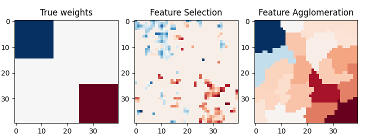
عكس التحويل لعرض النتائج على صورة

plt.close("all")
plt.figure(figsize=(7.3, 2.7))
plt.subplot(1, 3, 1)
plt.imshow(coef, interpolation="nearest", cmap=plt.cm.RdBu_r)
plt.title("True weights")
plt.subplot(1, 3, 2)
plt.imshow(coef_selection_, interpolation="nearest", cmap=plt.cm.RdBu_r)
plt.title("Feature Selection")
plt.subplot(1, 3, 3)
plt.imshow(coef_agglomeration_, interpolation="nearest", cmap=plt.cm.RdBu_r)
plt.title("Feature Agglomeration")
plt.subplots_adjust(0.04, 0.0, 0.98, 0.94, 0.16, 0.26)
plt.show()

محاولة إزالة المجلد المؤقت، لا تقلق إذا فشلت العملية

shutil.rmtree(cachedir, ignore_errors=True)

Related examples

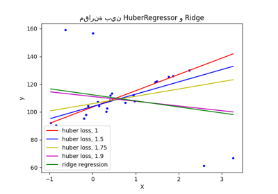
مقارنة بين HuberRegressor و Ridge على مجموعة بيانات تحتوي على قيم شاذة قوية

مقارنة بين HuberRegressor و Ridge على مجموعة بيانات تحتوي على قيم شاذة قوية

عرض توضيحي لتجميع هرمي منظم على صورة عملات معدنية

عرض توضيحي لتجميع هرمي منظم على صورة عملات معدنية

مطابقة متعامدة

مطابقة متعامدة

تجميع الميزات

تجميع الميزات